ENG | Center of Rotation from Matrix (by hand and SimPy)

Motivation

When working with image transformations, particularly in the context of keypoint detection and matching in computer vision, determining the precise center of rotation can be pivotal. This task, however, can present unexpected challenges. Despite exhaustive searches on platforms like StackOverflow, and even consulting advanced AI solutions like ChatGPT and Google Gemini, finding a straightforward answer proved elusive.

This exploration led to a journey through mathematical derivation, practical application, and the discovery of Python’s powerful SymPy library.

This article aims to share a concise, yet comprehensive guide to finding the center of rotation using (from) transformation matrices. Whether you’re dealing with a 2x3 or 3x3 matrix, the insights provided here will equip you with the tools needed to uncover the anchor point and angle of rotation.

Recovering the Center of Rotation: A Quick Guide

TL;DR: Here’s how to recover center (anchor, pivot point) and angle of rotation from 2x3 or 3x3 matrix, where translation is in the last column.

const double cosAlpha = m(0,0);
const double sinAlpha = m(1,0);
const double alphaRadians = atan2(sinAlpha, cosAlpha);
const double centerX  = ( m(0,2)*(1-cosAlpha) - m(1,2)*sinAlpha ) / (2*(1-cosAlpha));
const double centerY  = ( m(0,2) - centerX*(1-cosAlpha)) / sinAlpha;

You are welcome. Bye!

Oh, by the way … remember to check for division by zero when matrix is pure translation or identity.

Analytical Solution for Rotation Center in Transformation Matrices

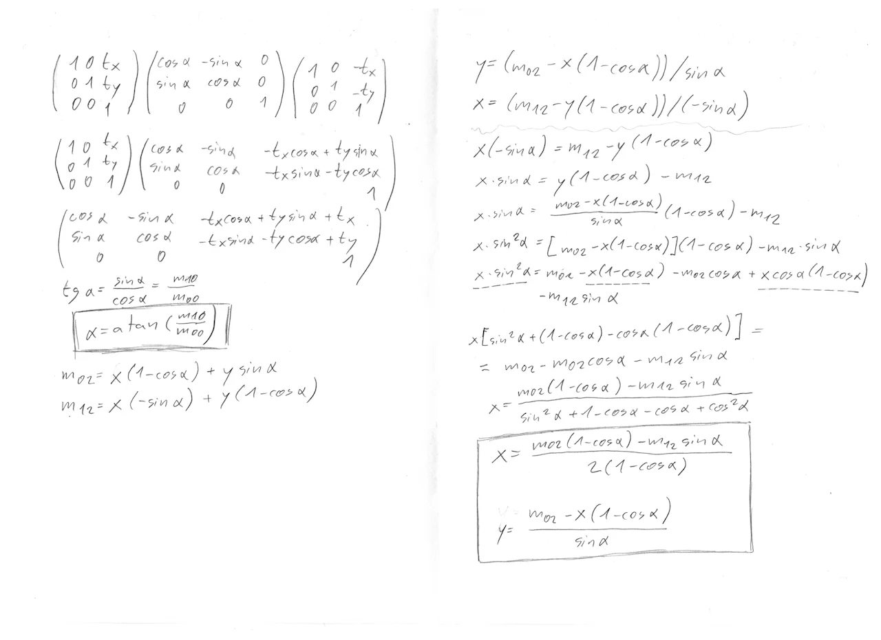
First we need to know how matrix for rotation around center is composed:

• Translate coordinates to rotation center (subtract coordinates of center)
• Perform rotation
• Translate coordinates back (add coordinates of center)

By multiplying these three matrices, we get matrix for rotation around center.

Then we can decode center of rotation from coeficients m02, m12 (last column).

I’m lazy to use TeX for equations today. Here’s the scan of solution.

Note that tx and x or ty and y are the same and both mean center of rotation.

Finding Equation for Rotation Center in Python

Matrix multiplication was done by hand.

I learned this trick from ChatGPT. SymPy is a Python library for symbolic mathematic. Note that sy.cos(a), x, a, m02 and so on are objects and eq1 basically holds parsed equation.

#!/usr/bin/env python3

import sympy as sy

# Define symbols
x, y, a, m02, m12 = sy.symbols('x y a m02 m12')

# Define equations
eq1 = m02 - (x * (1 - sy.cos(a)) + y * sy.sin(a))
eq2 = m12 - (x * (-sy.sin(a)) + y * (1 - sy.cos(a)))

# Solve the system of equations
solution = sy.solve((eq1, eq2), (x, y))

print(solution)

# Does not work, don't ask why
#solution[x].simplify()
#solution[x].simplify(trig=True)
#solution[y].trigsimp()

# Does work, don't ask why
simplified = {k: v.simplify() for k, v in solution.items()}
print("=== Hopefully simplified ===")
print(simplified)

print("=== Solved for y, then substitution ===")
solution_for_y = sy.solve(eq1, y)
print("y = ", solution_for_y)
eq3 = m12 - (x * (-sy.sin(a)) + solution_for_y[0] * (1 - sy.cos(a)))
solution_for_x = sy.solve(eq3, x)
print("x = ", solution_for_x)

Output with slightly modified formatting:

python ./sympy_solve2.py

{ x: -m02*cos(a)/(sin(a)**2 + cos(a)**2 - 2*cos(a) + 1) + m02/(sin(a)**2 + cos(a)**2 - 2*cos(a) + 1) - m12*sin(a)/(sin(a)**2 + cos(a)**2 - 2*cos(a) + 1), 
  y:  m02*sin(a)/(sin(a)**2 + cos(a)**2 - 2*cos(a) + 1) - m12*cos(a)/(sin(a)**2 + cos(a)**2 - 2*cos(a) + 1) + m12/(sin(a)**2 + cos(a)**2 - 2*cos(a) + 1) }

=== Hopefully simplified ===
{ x: (m02*cos(a) - m02 + m12*sin(a))/(2*(cos(a) - 1)), 
  y: (m02*sin(a) - m12*cos(a) + m12)/(2 - 2*cos(a))}

=== Solved for y, then substitution ===
y = [(m02 + x*cos(a) - x)/sin(a)]
x = [(m02*cos(a) - m02 + m12*sin(a))/(2*(cos(a) - 1))]

Going full Python (added 2024-03-21)

And we can do even better

import sympy as sp

# Define symbolic variables
tx, ty, a = sp.symbols('tx ty a')

# Define transformation matrices
Tr_minus = sp.Matrix([[1, 0, -tx],
                      [0, 1, -ty],
                      [0, 0, 1]])

Rot = sp.Matrix([[sp.cos(a), -sp.sin(a), 0],
                 [sp.sin(a), sp.cos(a), 0],
                 [0, 0, 1]])

Tr_plus = sp.Matrix([[1, 0, +tx],
                     [0, 1, +ty],
                     [0, 0, 1]])

M = Tr_plus * Rot * Tr_minus

print("M:    ", M)
m02, m12 = sp.symbols('m02, m12')
eq1 = sp.Eq(m02, M[0,2])
eq2 = sp.Eq(m12, M[1,2])
print("eq1:  ", eq1)
print("eq2:  ", eq2)

solution = sp.solve((eq1, eq2), (tx, ty))
simplified = {k: v.simplify() for k, v in solution.items()}
print("=== Hopefully simplified solution ===")
print(simplified)

M:     Matrix([[cos(a), -sin(a), -tx*cos(a) + tx + ty*sin(a)],
               [sin(a),  cos(a), -tx*sin(a) - ty*cos(a) + ty],
               [     0,       0,                           1]])
eq1:   Eq(m02, -tx*cos(a) + tx + ty*sin(a))
eq2:   Eq(m12, -tx*sin(a) - ty*cos(a) + ty)
=== Hopefully simplified solution  ===
{tx: (m02*cos(a) - m02 + m12*sin(a)) / (2*(cos(a) - 1)), 
 ty: (m02*sin(a) - m12*cos(a) + m12) / (2 - 2*cos(a))}

At least we have AI today and we can spend half hour to generate this Python script, instead of fourty minutes by doing this by hand. But I put it here, because it’ll be helpful next time.

Eigenvectors: An Alternative Approach

I had an idea to use Eigenvectors to find a solution. These vectors have their direction unchanged when they are multiplied by matrix. Eigenvalue specifies change of their length.

Rotation around point is rotation followed translation. Translation is encoded as a shear transform in higher dimension. Point which in center of rotation has coordinates [x,y,1] and they remain unchanged.

However, there are two key things to note about this approach:

1. There are three eigenvectors and eigenvalues, two solutions are complex. The real solution corresponds to an eigenvalue of 1.
2. The normalization step is crucial because the eigenvectors are initially in homogeneous coordinates (represented as [x, y, w]), where w is a scaling factor and they are normalized to unit lenght. Dividing each component by w ensures we recover the “proper” coordinates ([x, y, 1]) of the center of rotation.

    print("\033[33;1mOutput:\033[0m")
    print("Transformation matrix decoded by cv2.findHomography(pts1, pts2, ...)")
    print(M)
    eigenvalues, eigenvectors = np.linalg.eig(M)
    # Filter to keep only real eigenvalues and eigenvectors (should be where
    # eigenvalue is close to 1 and if real_eigenvectors[2] is not close to zero)
    real_indices      = np.isreal(eigenvalues)
    real_eigenvalues  = eigenvalues[real_indices].real
    real_eigenvectors = eigenvectors[:, real_indices].real
    print("Real Eigenvalues:\n",  real_eigenvalues)
    print("Real Eigenvectors:\n", real_eigenvectors)
    print("All  Eigenvalues:\n",  eigenvalues)
    print("All  Eigenvectors:\n", eigenvectors)
    real_eigenvectors = real_eigenvectors / real_eigenvectors[2]
    print("Eigenvector normalized:\n", real_eigenvectors)
    print("Estimated center of rotation [{}, {}]".format(real_eigenvectors[0][0], real_eigenvectors[1][0]))
    est_rotation = np.arctan2(-M[1][0], M[0][0])
    print("Estimated angle of rotation  {}".format(est_rotation / np.pi * 180.0))

    cos_a = M[0][0]
    sin_a = M[1][0]
    cx = M[0][2]*(1-cos_a) - M[1][2]*sin_a
    cx /= 2*(1-cos_a)
    cy = ( M[0][2] - cx*(1-cos_a) ) / sin_a
    print("CX={}".format(cx))
    print("CY={}".format(cy))

Output with slightly modified formatting:

Input:
center_x=306.000000, center_y=336.000000, angle=53.130102 clockwise
Transformation matrix applied in image:
[[   0.6    0.8 -146.4]
 [  -0.8    0.6  379.2]]

Output:
Transformation matrix decoded by cv2.findHomography(pts1, pts2, ...)
[[ 6.00049403e-01  8.00081887e-01 -1.46520193e+02]
 [-8.00007900e-01  6.00103906e-01  3.79495598e+02]
 [ 2.54400882e-08  1.75551165e-07  1.00000000e+00]]

Real Eigenvalues:
 [1.00006682]
Real Eigenvectors:
 [[0.67336197]
  [0.7393097 ]
  [0.00219869]]
All  Eigenvalues:
 [0.60004324 + 0.80002229j   0.60004324 - 0.80002229j   1.00006682 + 0.j ]
All  Eigenvectors:
 [[-7.07140448e-01 + 0.00000000e+00j   -7.07140448e-01 - 0.00000000e+00j   6.73361968e-01 + 0.j]
  [-1.56417959e-05 - 7.07073113e-01j   -1.56417959e-05 + 7.07073113e-01j   7.39309695e-01 + 0.j]
  [-1.15135555e-07 + 8.00499000e-08j   -1.15135555e-07 - 8.00499000e-08j   2.19868520e-03 + 0.j]]
Eigenvector normalized:
 [[306.25665202]
  [336.25081716]
  [  1.        ]]
Estimated center of rotation [306.25665202043785, 336.25081716076375]
Estimated angle of rotation  53.12810956081744

CX=306.2861253898095
CY=336.27106941866657

When working with OpenCV always double-check …

• if y has meaning of up or row/down
• if angle of rotation is clockwise or counter-clockwise
• if coordinates are in order [row,column] or [x,y]
• consider cv2.estimateAffinePartial2D instead of cv2.findHomography

Good luck and have fun!

Geometric solution

• See Mammoth Memory - How do you find the center of rotation?

Conclusion

Which solution is better? Curiously eigenvectors seem slightly superior. Why? I guess that it’s because matrix returned by cv::estimateAffinePartial2D contains scaling (although small) and analytical solution is more sensitive.

While challenges were encountered (particularly with sympy and sign errors in handcrafted solution) the process was ultimately rewarding.

It was also nice test of AI. It failed proposing eigenvectors as solution to C = M * C, where C is a center of rotation, but was very happy when I proposed finding eigenvectors and helped with Python code a lot.