ENG | Introduction to Transformation Matrices, part I
Introduction
Before diving into matrix transformations, it’s important to have a basic understanding of linear algebra, vector and matrices.
Vectors are fundamental mathematical objects that play a crucial role in linear algebra, physics, computer graphics, and many other fields. In this article, we’ll explore the concept of vectors, their properties, and their relationship with matrices.
If you familiar with basic, skip article to Matrix and Vector Multiplication Analysis, part about of vector is there mostly because of:
This article was written partly in October 2018, partly in summer 2022. Then it was revised and extended by Claude.AI in March 2024 - it basically wrote the whole vector part.
Vector
A vector is a mathematical entity that has both magnitude and direction. It can be represented geometrically as an arrow with a specific length and orientation in space. They can placed anywhere for visual clarity, but their origin is not defined. In two-dimensional (2D) space, a vector is defined by its x and y components, while in three-dimensional (3D) space, it has x, y, and z components.
Vectors are often denoted using bold letters or an arrow above the letter $\vec{a}$ and the components of a vector in 3D space can be written as $\vec{a} = (a_x, a_y, a_z)$.
Vector Operations
There are several operations that can be performed on vectors, including addition, subtraction, scalar multiplication, and various products.
Vector Addition and Subtraction
Vector addition and subtraction are performed component-wise. For two vectors $\vec{a}$ and $\vec{b}$, their sum and difference are defined as:
\[\vec{a} + \vec{b} = (a_x + b_x, a_y + b_y, a_z + b_z)\] \[\vec{a} - \vec{b} = (a_x - b_x, a_y - b_y, a_z - b_z)\]TODO: image or animation
Scalar Multiplication
Scalar multiplication is the multiplication of a vector by a scalar value (a real number). For a vector $\vec{a}$ and a scalar $k$, the scalar multiplication is defined as:
\[k \vec{a} = (k a_x, k a_y, k a_z)\]Scalar multiplication changes the magnitude of the vector but not its direction.
Dot Product
The dot product, also known as the scalar product, of two vectors $\vec{a}$ and $\vec{b}$ is a scalar value defined as:
\[\vec{a} \cdot \vec{b} = ||\vec{a}|| \ ||\vec{b}|| \cos\theta\]where $\theta$ is the angle between the vectors, $||\vec{a}||$ and $||\vec{b}||$ are the magnitudes (lengths) of the vectors.
Alternatively, the dot product can be calculated using the vector components:
\[\vec{a} \cdot \vec{b} = a_x b_x + a_y b_y + a_z b_z\]The dot product has several important properties and applications, such as determining the angle between two vectors, or projecting one vector onto another.
Cross Product
The cross product, also known as the vector product, is an operation that is defined only in three-dimensional space. The cross product of two vectors $\vec{a}$ and $\vec{b}$ is a vector $\vec{c}$ that is perpendicular to both $\vec{a}$ and $\vec{b}$, with a magnitude equal to the area of the parallelogram formed by $\vec{a}$ and $\vec{b}$ which is $||\vec{a}|| \ ||\vec{b}|| \sin\theta$. Direction follows right hand rule.
The cross product is calculated using the determinant:
\[\vec{a} \times \vec{b} = \begin{vmatrix} \vec{i} & \vec{j} & \vec{k} \\ a_x & a_y & a_z \\ b_x & b_y & b_z \end{vmatrix} = (a_y b_z - b_y a_z) \vec{i} + (a_z b_x - b_z a_x) \vec{j} + (a_x b_y - b_x a_y) \vec{k} +\]where $\vec{i}$, $\vec{j}$, and $\vec{k}$ are the unit vectors along the x, y, and z axes, respectively.
The cross product has several important applications, such as calculating the normal vector of a plane (it’s perpedicular to both input vectors). In physics, cross products usually emerges when one vector is pseudo-vector encoding axis of rotation rather then direction (angular momentum, torque, Lorentz force, …).
If two vectors are parallel or anti-parallel $\vec{a} \times \vec{b} = 0$
Matrices
Matrices are rectangular arrays of numbers used to represent linear transformations. A matrix with m rows and n columns is denoted as an m×n matrix.
In this article, we’ll explore why matrices are essential tool used in computer graphics.
Linear transformations include mirroring, rotation, scaling, and shearing. They can be represented by a 2x2 matrix in 2D, and by 3x3 matrix in 3D space. Keep in mind that first number is number of rows and second is number of columns.
2D Linear Transformations
In the context of linear transformations, we express coordinates as pairs of $x$ and $y$ components. Linear transformations can be represented by calculating new $x’$ and $y’$ coordinates:
\[\begin{align*} x^\prime =& x \cdot m_{00} + y \cdot m_{01}, \\ y^\prime =& x \cdot m_{10} + y \cdot m_{11} \end{align*}\]where $m_{ij}$ are the transformation parameters.
Using vector/matrix notation, we can express the entire transformation as:
\[\begin{bmatrix} x' \\ y' \end{bmatrix} = \begin{bmatrix} m_{00} & m_{01} \\ m_{10} & m_{11} \end{bmatrix} \begin{bmatrix} x \\ y \end{bmatrix}\] \[v^\prime = M \cdot v\]3D Transformations
Let’s make it more complicated.
In 3D, we need 3-element vectors $(x, y, z)$ and a 3x3 matrix for linear transformations. However, translation is not a linear transformation (and needs 3x4 matrix) and projection neither (needs 4x4 matrix). They are linear in four dimensions.
Points and vectors behave differently under translations. Vectors are immune to translation, they represent directions and relative displacements, but they have no position. On the other hand, points are affected by translations, and their positions change accordingly. This difference arises because points represent absolute locations or coordinates.
To handle both points and vectors in the same transformation framework, homogeneous coordinates are used. Homogeneous coordinates introduce an additional dimension (typically denoted as $w$) to represent points and vectors in a unified way.
- For points ($w = 1$), the translation components in the fourth column of the matrix get added to the x, y, z coordinates, effectively translating the point (skew transform in upper dimension)
- For vectors ($w = 0$), the fourth column has no effect, as anything multiplied by 0 becomes 0, leaving the vector’s direction and magnitude unchanged under translation.
The $w$ coordinate together with fourth row also has a special use in perspective projection - first $-z$ is copied to $w$ and then all coordinates are divided by $w$ because multiple points in 3D are projected to a single point in 2D. We will get there (in a separate article I guess)
This unified treatment of points and vectors using homogeneous coordinates is a powerful tool in computer graphics, robotics, and other fields dealing with spatial transformations.
Side Note: Types of Transformation
- Linear Transformation: mirroring, rotation, scaling, and shearing. They preserve origin and parallel lines. They are represented by 3x3 matrix for 3D space.
- Affine Transformation: Linear transformations plus translation. They do not preserve origin. They are represented by 4x4 (or 3x4) matrix for 3D space.
- Projective Transformation: Affine transformations plus perspective projection. Line parallelism and origin are not preserved. 4x4 matrix for 3D space.
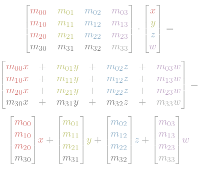
Matrix vector multiplication
The multiplication of a matrix $A$ and a vector $\vec{x}$ is defined as:
\[M \vec{v} = \begin{bmatrix} m_{00} & m_{01} & \cdots & m_{0j} \\ m_{10} & m_{11} & \cdots & m_{1j} \\ \vdots & \vdots & \ddots & \vdots \\ m_{i0} & m_{i1} & \cdots & m_{ij} \end{bmatrix} \begin{bmatrix} v_0 \\ v_1 \\ \vdots \\ v_i \end{bmatrix} = \begin{bmatrix} m_{00}v_1 + m_{01}v_2 + \cdots + m_{0j}v_i \\ m_{10}v_1 + m_{11}v_2 + \cdots + m_{2j}v_i \\ \vdots \\ m_{i0}v_1 + m_{i1}v_2 + \cdots + m_{ij}v_i \end{bmatrix}\]Matrix and Vector Multiplication Analysis
Many presentations introduce examples of translations, rotations, and other transformations across several PowerPoint slides. Let’s try a different approach by analyzing the multiplication of a 4x4 matrix and a 4x1 matrix (column vector) to understand the concept. This will allows us to synthetise transformation matrices later without need to memorize them. This example hopefully sheds some light on the previous chapter.
From a definition, the result of matrix multiplication is a matrix where the element in row i and column j is dot product of the row i of the first matrix and column j of the second matrix. The number of columns of the first matrix must match the number of rows of the second one.
Note that when we multiply matrix and, for example, unit vector x, red numbers in the matrix will define vector into which unit vector x will be transformed. The same is true for other unit vectors.
Example:

Unit vector $x$ is transformed into
\[\begin{align*} x^\prime &= \cos(30^{\circ}) = \sqrt3 / 2, \\ y^\prime &= \sin(30^{\circ}) = 1/2 \end{align*}\]Unit vector $y$ is transformed into
\[\begin{align*} x^\prime &= -\sin(30^{\circ}) = -1/2, \\ y^\prime &= \cos(30^{\circ}) = \sqrt3/2 \end{align*}\]- Unit vector $z$ is unchanged (but multiplied by zero)
Unit vector $w$, borrowed from 4th dimension, is transformed into
\[\begin{align*} x\prime &= 2, \\ y\prime &= 1, \\ w\prime &= 1 \end{align*}\]and causes translation. For this reason, points have
w=1, while vectors havew=0and are immune to translation. Actually points are on a planew=1and 4th dimension is skewed (shear transform).
Now we can multiply transformed unit vectors by a scalars which are components of the vector we want to transform and add them together.

Composition of Transformations
If the second matrix is not a column vector but a transformation matrix, it can be interpreted as four column vectors representing the basis of coordinate system.
The first matrix then transforms these basis vectors individually, effectively transforming the entire coordinate system.
Keep in mind that number of rows in the second matrix has to match number of columns of the first matrix.
For column vectors, which are more common in 3D computer graphics, transformations are applied from right to left. In the case of row vectors, transformations are applied from left to right, and the matrices are diagonally mirrored (a process known as transposition, with translations located in the last row).
Transformation of Normal Vectors
It’s important to know that scaling and mirroring normal vectors using the same transformation matrix is not possible, as it would make them no longer perpendicular to surfaces.
To address this, we can use the inverse transpose of the transformation matrix for transforming normal vectors, ensuring they remain perpendicular after the transformation.
TODO: image showing that normal vectors are no longer perpedicular to lines/surfaces, side note about fixing this TODO: show inverse transpose matrix
Technical note about different notations
Even if different libraries might be consistent in using column vectors, a memory layout can differ. Eigen, by default, stores matrix column-by-column (m₀₀, m₁₀, …) which is OpenGL compatible, while other libraies may store them row-by-row (m₀₀, m₀₁, …). Memory layout is called row-major or column-major. This detail is usually hidden behind some access operator.
DirectX and OpenGL use notation with row vectors. To be precise, OpenGL does not care. It only states that translation is elements 12,13,14 of linear array and transforms are put in stack (OpenGL2) or composed inside shaders where notation depends on which side of matrix the vector is (OpenGL3 and newer).
In evil cases, left-handed coordinate systems are used rotations are specified in clock-wise direction (x towards y axis, but y is pointing down) or their usage is not consistent (welcome to realm of OpenCV)
Undoing transformations
To undo the transformation, we use the inverse matrix.
Calculating the inverse matrix can be done by hand (using the Gauss elimination method) or by employing a non-trivial algorithm that requires several steps and involves calculating many determinants. Computation complexity is high.
Determinant
The determinant of a transform matrix is equal to a signed volume of parallelepiped defined by columns of the matrix. For a rotation matrix, the determinant is equal to one, for the reflection matrix it is minus one. When the determinant is zero, we lose one or more dimensions and the inverse matrix cannot be found (for example, when projecting 3D space onto a plane), because this transformation is inherently irreversible.
Great video explanation of Why is the determinant like that? which goes deep into problematic and determinant signs and higher dimesions.
Next part is work in progress for two years. There is also part 2 which needs to be modified slightly for this blog about model->view->camera transforms.
Important stuff ends here, notes can be skipped.
NOTES
Note about direct placement of objects
We don’t need to memorize the appearance of a rotation matrix. We can construct it directly, as should be evident from the illustrated example mentioned earlier.
Understanding the meaning of matrix columns is used for placing parts into flanges in the collision model (although this feature is not used today). Attachment points are defined by a coordinate of the flange center, the vector pointing forward into the hole, and the vector defining the up direction. Matching parts have the same vectors. We can get the vector pointing right by taking the cross product of the forward and up vectors and then normalizing the result. If the up is not required to be perpendicular to forward, we can find a new up2 by taking the cross product of the “right” and “forward” vectors and normalizing the result consecutively.
Now we have three orthogonal vectors defining orientation and origin vector defining position. To match the orientation and position of a part to a flange, we must multiply the matrix of a flange (transforming the reference/world coordinate system into flange’s) and invert the matrix of the part (transforming the part into the reference/world coordinate system).
TODO: image, remove Tescan specific stuff
Note about rotations and their interpolation (quaternions, rotors, etc.)
Note: there’s no simple way how to find the axis and angle of rotation between two transformation matrices or how to interpolate rotation. For this purpose, quaternions are often used (or rotors from geometric algebra, or complex numbers in 2D). Another reason for using quaternions is that they are easy to normalize and more resistant to rounding errors when stacking multiple rotations together. However, they are less versatile and matrix-vector multiplication is cheaper than quaternion-vector-quaternion multiplication (though matrix-matrix multiplication is more expensive than quaternion-quaternion multiplication). Quaternions and rotors are numerically similar (though their definitions and algebra behind them are different — quaternions are highly abstract and difficult to comprehend, while geometric algebra is just very challenging). Both quaternions and rotors are easy to construct from the axis of rotation and angle, or vice versa, decomposed. They are numerically stable (Euler angles have gimbal lock problem, matrices can’t do 180 degree rotation)
TODO: add example of quaternion rotation interpolation, perhaps another file
Applications of quaternions (and GA)
- Composing many tiny rotations (better numerical stability, easier to normalize)
- Finding angle and axis between two rotations
- Interpolation between two rotations - however neither complex numbers nor quaternions can be interpolated directly (they must have unit lenght, but normalizing is not enough if we want constant angular speed - we must interpolate angle, and, in 3D, we have to find axis of rotation too)
- Generating random orientation: random axis of rotation and random angle. To make random axis of rotation, normalize random point inside a unit sphere. To generate that point, create a random point inside cube and reject it if the distance from origin exceeds one.
- Trackball rotation: A quaternion is constructed from two points on a sphere. This technique is used for intuitive changes in rotation, such as mouse dragging a virtual trackball. Commonly used in 3D software for user interaction.
- Quaternions have advantage of numberical stability and they can be used for spacecraft orientation control
Note about geometry algebra (off-topic)
Geometric algebra is a mathematical framework that unifies various concepts from physics and geometry, making some processes more intuitive and elegant. It incorporates scalars, imaginary numbers, quaternions, and vectors, while distinguishing between different types of vector operations. For instance, the cross product, which only exists in 3D, is replaced by the more general wedge product. This results in an oriented plane in 2D rather than a vector in the 3rd dimension. Pseudovectors that encode axis of rotation and angle are replaced by bivectors, such as angular momentum in physics. It provides a unified language for expressing geometric transformations, making it easier to manipulate and reason about them.
Geometric algebra also helps clarify some concepts in physics, by explaining why certain vectors are multiplied by dot or cross product and allowing for a distinction between true vectors and those representing axes of rotation.
In 2D space, geometric algebra includes scalars, two vector components e1, e2, and a bivector e12, which has properties similar to imaginary numbers and encodes an oriented surface. In 3D space, geometric algebra consists of scalars, three vector components, three bivectors (e12, e13, e23) that correspond to i, j, and k in quaternions, and a trivector e123 representing oriented volume.
Finally, there is a third product in geometric algebra called the geometric product, which is the sum of the dot and wedge products.
Geometric algebra can be used in various fields, such as physics, computer vision, robotics, and signal processing. It allows for more intuitive and compact formulations of equations and algorithms in these fields.
In robotics, geometric algebra can be employed to describe the kinematics and dynamics of robotic systems, leading to more efficient and accurate control algorithms.
Clifford algebra, a generalization of quaternions and geometric algebra, has found applications in quantum mechanics, relativity, and other areas of theoretical physics. Clifford algebra provides a natural way to represent and manipulate geometric entities like vectors, bivectors, and spinors.
TODO: camera placement (maybe in coord-sys-camera)
TODO: example: point centered rotation
TODO: axis, angle rotation
TODO: mention euler angles somewhere
TODO: more about matrix inversion (rotation, translation -> translation rotation)
TODO: Julia and Python examples
Useful links
- Introduction to linear algebra, matrices, dot and cross products and more (series, 3Blue1Brown): https://www.youtube.com/watch?v=fNk_zzaMoSs&list=PLZHQObOWTQDPD3MizzM2xVFitgF8hE_ab
- Matrices and operations https://www.mathsisfun.com/algebra/matrix-index.html
- Brief introduction to geometric algebra for curious people (Marc ten Bosch): https://marctenbosch.com/quaternions/
- Very long series dedicated to geometric algebra (Mathoma): https://www.youtube.com/playlist?list=PLpzmRsG7u_gqaTo_vEseQ7U8KFvtiJY4K
- Introduction to linear algebra, matrices, dot and cross products and more (video series, 3Blue1Brown)
- Matrices and operations (article)
- Brief introduction to geometric algebra for curious people (Marc ten Bosch)
- Very long series dedicated to geometric algebra (Mathoma)