ENG | Advanced Use of the Logarithmic Slide Rule: Solved Word Problems
Introduction
Starting with simple examples and moving towards more complex ones is a widely accepted teaching method. However, I consider this approach to be somewhat redundant for our purposes, as the fundamentals of slide rule operations are extensively documented elsewhere (e.g. Slide Rule Calculations by Example)
The selected examples stem from intriguing discussions I’ve had with colleagues at work, which sparked my curiosity to explore these topics further.
Hopefully these two examples covered all common scales except trigonometric scales, cubic scales and quadratic scales which are easy to use.
As always I believe this article is somewhat unique.

Having a slide rule in your hands is almost essential for following along. The article assumes familiarity with the device, using it to navigate through calculations that are both intriguing and applicable. If you’re not ready to use a slide rule for these examples, you might miss out on the practical insights offered. Or you may try virtual Slide Rule Simulator
I’d also like to recommend to read article about Reinventing logarithms and slide rule
Example 1: Hard Drive Life Expectancy
Background
We often see hard drives advertised with a lifespan measured in “MTBF” (mean time between failures). While this number might sound impressive, it’s important to understand what it really means.
Consider the following example. We have hard drive that specifies 600000 hours between failures (MTBF) or mean time to failure (MTTF). This says that if we have 1000 hard drives, running for 600M hours total, there will be likely 1000 failures. It does not mean that all drives will fail, because failed ones will be replaced, but their average life expectancy.
In real life, hard drives tend to fail either early or after several years due to wear. If they have MTBF specified as high as 1.2 million hours, it looks good, but 137 years of continuous operation? I guess that drives that fail very early are excluded and statistics are made from hard drives that did not die in the first weeks and that do not run longer than months, because testing them for longer, before they are released to market is not realistic (no one will wait for 100 years). It’s akin to estimating human life expectancy based solely on mortality of people in twenties (11 deaths per 1000 according to WHO. This would suggest that people live roughly thousand years and actually even longer in developed countries.
For the sake of simplicity, we’ll assume that hard drives fail randomly, at constant rate, regardless of their age. With that assumption we can say that chance of failure is constant per any time unit and number of working drives decreases exponentially.
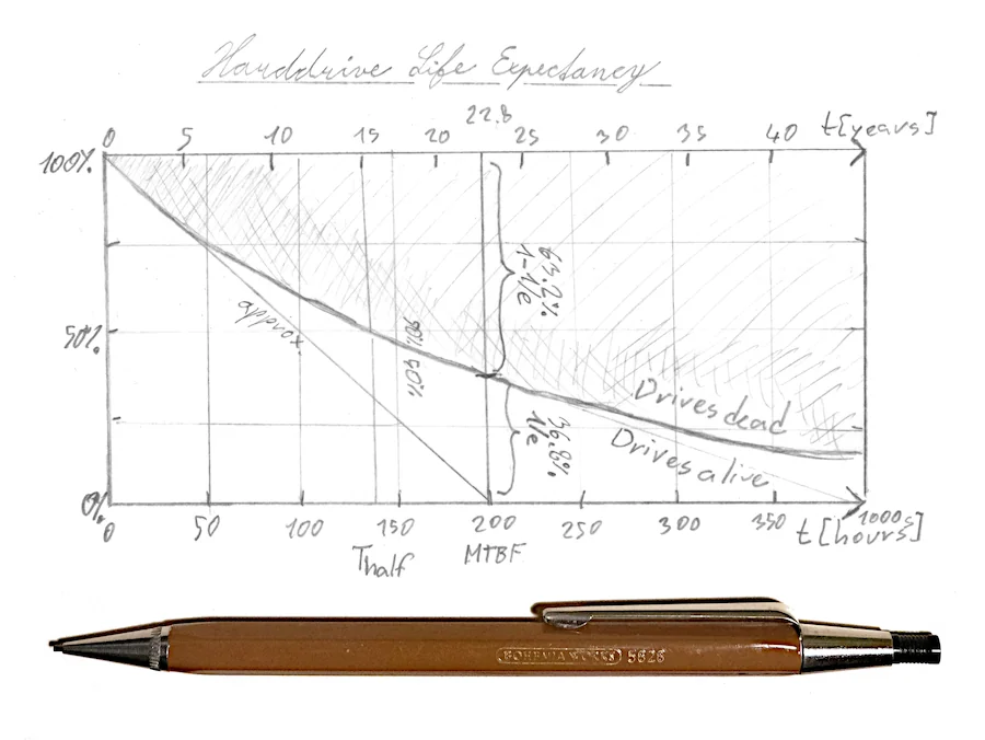 Harddrive life expectancy graph for 200000 hours MTBF
Article How Long Do Disk Drives Last? from Backblaze shows that chance of failure significantly increases after five years of non-stop service and there’s a article Estimating Drive Reliability in Desktop Computersand Consumer Electronics Systems from Seagate which mentions influence of temperature.
We have following questions:
1.1 How many years is 200k or 600k hours?
1
2
3
4
5
julia> 365*24
8760

julia> 200000/8760
22.831050228310502
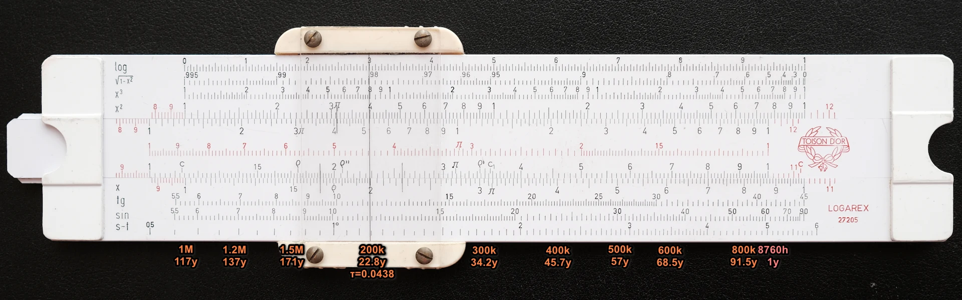 Conversion between years and hours. As you can see slide rule can be used for proportions or unit conversions. Parallel computing! Click for higher resolution.
We aligned C,D scales moving slider to the left - this allows us to convert MTBF (time constant τ) in hours not only to MTBF in years, but also to decay constant λ=±1/τ (-1/MTBF) which is slope at time zero. It also gives “nicer” numbers such as 0.0438 instead of 22.831050.
1.2 What’s the chance that hard drive fails in one year (annualized failure rate, AFR)?
Equation for anualized failure rate is $ 1-e^{\left(-{8760/MTBF}\right)} $ or just $ 8760/MTBF $, because slope of the function is nearly linear, when MTBF is high. In time equal to MTBF, ratio of working drives is $ e^{-1} = 1/e = 0.367 $ and ratio of failed drives is $ 1-e^{-1} = 1-0.367 = 0.632 $.
1
2
3
4
5
julia> 1-exp(-8760/200000)
0.04285463259510358

julia> 8760/200000
0.0438
In this case, if we use linear approximation, error is roughly 2% for the first year.
Oh, by the way … this is much more obvious if we use years and healthy drives. If ratio of working hard drives drops to 1/e in 22.83 years, in one year, it drops by
\[1/\sqrt[22.83]{e} = 1/e^{\left({1/22.83}\right)} = e^{\left({-1/22.83}\right)} = e^{-0.0438} = 0.9571\]In other words, we are searching for a number which we have to multiply by itself 22.83 times to get 1/e.
Duplex slide rule with LL0/e^-x scales
Curiously, we can find ratio of working drives on typical duplex slide rule instantly by a single cursor move:
- Set cursor to 2.28 on CI scale (time constant 22.8 years)
- Unnecessary: Read 4.38 (0.0438) on C scale (1/20 is 0.05 to keep track about order of magnitude) to get exponent (you don’t need to know it) or decay constant if you are interested. It’s a slope of function at t=0.
- Look up value above on scale labeled e^-0.01x as 0.9572
- Subtract 1-0.9572 manually to get 0.0428
Note that using CI scale is not necessary. We can use distance between 1 and 2.28 on C,CI,CF or even CIF scale, they are the same. Important is that we want to use this distance leftwards.
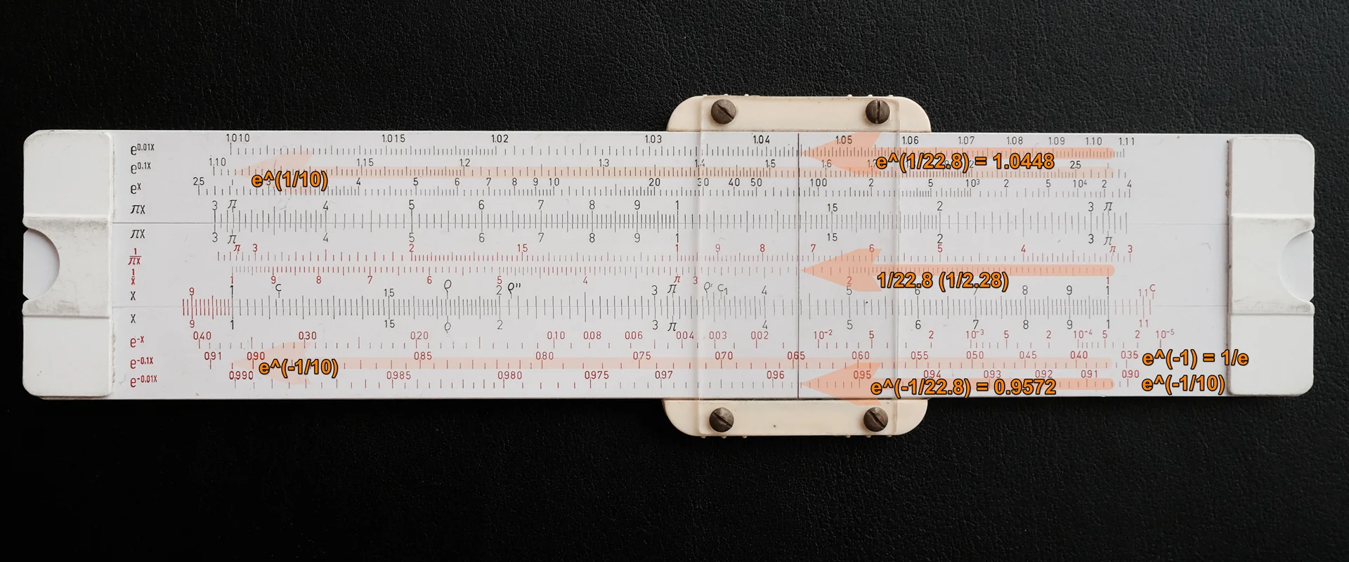 Finding 22.8th root of 1/e (0.9572) and e (1.0448).
Darmstadt slide rule (or some scholar types)
Darmstadt type slide rules are common in Europe. They do not have LL0 scales, just LL scales on the back of slider. Another distinctive feature is P scale.
We need to do some mental exercise here. Our slide rule cannot deal with exponential decline, but only with exponential growth. So let’s revert the time axis. We have e (2.71) times more working drives 22.8 years ago. Question is number of working drives we had one year ago relatively to today.
Sadly, inverting numbers close to one can lead to a loss of accuracy, which is why I chose an MTBF of 200,000 hours for this example.
- Align C=1 against D=2.28 (22.8 years)
- Turn slide rule
- Read 1.0448 against hairline. Why? If we go one row up from 2.71 to 1.05, its $e^{1/10}$. Now, if we go 2.28 left it’s $ e^{1 / (10 \cdot 2.28)} $. This means we had roughly 1.045 times more working drive year ago.
- Now we evaluate 1/1.045=0.96 - number of working drives next year.
- Subtract 1-0.96 which is 0.04 - number of failed drives next year.
Rietz or Mannheim slide rule (or others without LL1, LL2 scales)
We need different approach. We know that number of hard drives increases e times in 22.8 years backwards in time. In one year it’s 22.8th root of e.
Trust me it’s easier than original formula which needs avoiding logarithms of negative argument, evaluating $ 10^{-0.019} $ - this article is long as it is already.
\[\begin{align*} \sqrt[22.8]{e} &= x \\ e^{1/22.8} &= x \\ \log e^{1/22.8} &= \log x \\ \frac{1}{22.8} \log e &= \log x \\ 0.43429 / 22.8 &= \log x \\ \log x &= 0.019 \\ x &= 10^{0.019} \\ x &= 1.045 \end{align*}\]- $ \log_{10}e = \log_{10}2.72 = 0.434 $ using D,L scales (e is likely not marked, but there might be table of constants with value $ \log e=0.43429 $ on the back side.
- $ 0.434/22.8 = 0.434*0.0438 = 0.019 $ (use C,D scales)
- $ 10^{0.019}=1.045 $ (cursor to L=0.019, read 1.045 on C or D scale assuming they are aligned), this is relative number of working drives year ago
- $ 1/1.045=0.9575 $ (cursor to L=0.019 between ticks, read 0.9575 between 0.955 and 0.96 tick on CI scale), relative number of working drives next year
- $ 1-0.9575=0.0425 $, failed drives next year (annualized failure rate)
1.3 In what time period 10% or 50% of hard drives fails?
Duplex slide rule
We randomly found that we can use just a cursor movement. In one year 0.9572 drives survives. Now we want to measure distance to 0.9 and convert it to years. Sadly LL scale wraps around and on some slide rules it’s not on the same row. We have to set cursor to 0.9572 on LL03 scale and align 10 on C scale with cursor. Then we can read on C scale that below LL02=0.9 is C=2.4. Let’s verify it:
1
2
julia> 0.9572^2.4
0.90033981466062
We can use slide rule to the maximum. Remember that distances between numbers are the same for scales $ x, 1/x, \pi x, 1/\pi x $. We can align cursor with end of scale (where C=1 or 10) and align 2.28 on CF scale with cursor. Now we can use cursor for direct conversion between time (on CF scale) and fraction of drives alive! At time 1 we have 0.9572 (95.7%) drives alive and in 10 years we have 65% drives alive. To get time where 90% of drives are alive we move cursor to e^-0.01x=0.9 and we read 2.4 years on CF scale. To get “Half life” we move cursor to e^-0.1x=0.5 and read 15.8 years. To get number of drives alive after 22.8 years we set cursor to 22.8 on CF scale and read 1/e as expected.
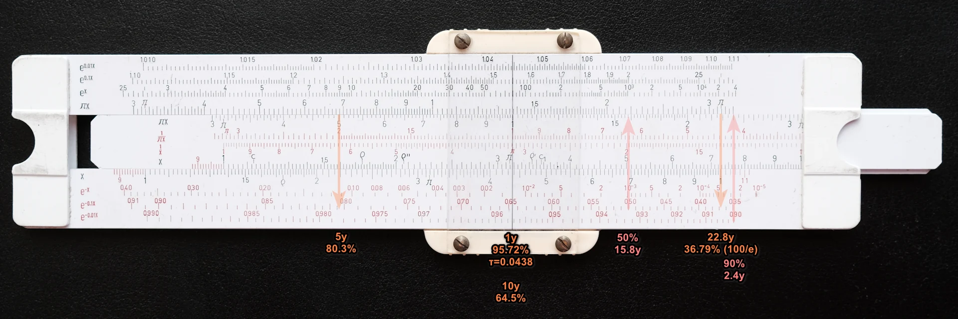 Direct conversion between time and percents of drives alive.
Darmstadt slide rule
Here it’s complicated and I would not be able to do it without using duplex slide rule first. We want to measure distance from 1/0.9572=1.0448 (tick before 1.045) to 1/0.9=1.111.
Basically ratio of drives alive year ago and time from which number of drives alive dropped to 90%.
I suggest turning the slider to it’s back side.
Sometimes slide rules have extended scales and 1.11 is on the same row. Then it’s quite obvious. Sometimes scale wraps around at 1.105. Then 1.0448 on LL scales must be aligned with 10 on D scale, and result is below 1.11 on LL scales. It’s 2.4.
Alternative
Without turning slide:
- Set 1.0448 against hairline. Read 2.28 on D scales against 1 (or against 10) on C scale
- Set 1.111 against hairline. Read 0.95 or 9.5 on D scale.
- Divide 2.28 by 0.95. It’s roughly 2.4.
Here I gave up dealing with orders of magnitude.
1
2
julia> log(1.111)/log(1.0448)
2.401810813304384
It’s very easy to make mistake when locating 1.1 or 1.111
Rietz slide rule
Relation between LL scales and D scale is natural logarithm with base $ e $ while relation between D and L scale is decadic logarithm with base 10
- $ \log 1.110 =0.045 $, 1/0.9 times more alive unkown time ago
- $ \log 1.045 =0.019 $, 1/(1-AFR), alive year ago
- $ 45/19=2.37 $
Or alternatively
- $ \log 0.9 = 0.954-1 = -0.046$, 90% survives unknown time
- $ \log 0.957 = 0.982-1 = -0.018, $ 1-AFR survives one year
- $ 46/18=2.55 $
Note that example with Rietz slide rule (25cm long scales) uses reading of logarithms of small numbers located just 4.75mm and 11.25mm away from zero trying to guesstimate values in between ticks that are 0.5mm apart.
Again. Without trying to simplify this and challenge myself to use more and more rudimentary slide rule and finding alternatives I probably would not be able to do this.
Bonus
1
2
3
4
5
6
7
8
9
10
11
12
13
14
15
16
17
18
using DataFrames

mtbf_hours = [200000, 300000, 400000, 500000, 600000,
              800000, 1000000, 1200000, 1500000, 2000000]
mtbf_years = mtbf_hours ./ 8760
afr = 1 .- exp.(-1 ./ mtbf_years)
fr5 = 1 .- (1 .- afr).^5

df = DataFrame(
  "MTBF [hours]"=> mtbf_hours,
  "MTBF [y]"  => round.(mtbf_years, sigdigits=3),
  "AFR [%]"   => round.(afr .* 100, sigdigits=2),
  "5y FR"     => round.(fr5 .* 100, sigdigits=2),
  "5% ☠ [y]"  => round.(-mtbf_years .* log(0.95), sigdigits=3),
  "10% ☠ [y]" => round.(-mtbf_years .* log(0.90), sigdigits=3),
  "50% ☠ [y]" => round.(-mtbf_years .* log(0.50), sigdigits=3),
)
println(df)
1
2
3
4
5
6
7
8
9
10
11
12
 MTBF [hours]  MTBF [y]  AFR [%]  5y FR    5% ☠ [y]  10% ☠ [y]  50% ☠ [y]
-------------------------------------------------------------------------
       200000      22.8     4.3      20.0      1.17       2.41       15.8
       300000      34.2     2.9      14.0      1.76       3.61       23.7
       400000      45.7     2.2      10.0      2.34       4.81       31.7
       500000      57.1     1.7       8.4      2.93       6.01       39.6
       600000      68.5     1.4       7.0      3.51       7.22       47.5
       800000      91.3     1.1       5.3      4.68       9.62       63.3
      1000000     114.0     0.87      4.3      5.86      12.0        79.1
      1200000     137.0     0.73      3.6      7.03      14.4        95.0
      1500000     171.0     0.58      2.9      8.78      18.0       119.0
      2000000     228.0     0.44      2.2     11.7       24.1       158.0
Table shows mean time between failures, anualized failure rate and ratio of drives that fail in 5 years. Then it shows how many years it takes for N-percents of drive to fail (50% is half-life).
So even if drive has specified mean time between failures as high as 600000 hours, there’s a 7% chance of failure in 5 years, and in 7 years chance of failure is 10%. Good luck without backups! Also note that in real world failure rate increases with temperature and hard drive’s wear, which we discussed in the introduction.
Summary
Calculations are surprisingly easy and very accurate on a duplex slide rule. Well, MTBF has one digit of precision anyways. If your hard drives fails it does not matter if there was a chance of 10%, 9.87% or 5% in five years. Not having backup is a russian roulette.
Darmstadt slide rule is quite unintuitive with changing $ y = e^{-x} $ to $ y = 1/e^x $ or $ 1/y = e^x $. It basically says that for each working drive today, we had 1.045 year ago and 2.72 hard drives 22.8 years ago - we basically turned exponential decay to exponential growth back in time. This conversion process offers a different perspective on how we can understand and manipulate data.
Example 2: Electron Speed vs. Accelerating Voltage.
This example needs slide rule with P scale.
Introduction
As we explore the acceleration of electrons to high speeds, it’s essential to consider relativistic effects. At velocities approaching the speed of light, classical mechanics gives way to relativistic physics, significantly affecting an electron’s mass and energy. These effects, governed by the Lorentz factor, $\gamma$, are crucial for accurately describing electron behavior under high accelerating voltages.
This understanding is not just academic; it underpins technologies ranging from particle accelerators to electron microscopes.
Potential energy of charged particle
Potential energy of charged particle in electric field is $ E_p = q \cdot \Delta U $ where q is charge and $ \Delta U $ is electric potential difference (accelerating voltage). Electron with charge $ e_0 = 1.602 \cdot 10^{-19} C $ and accelerated by electric field potential difference of $ 1V $ has energy
\[E_p = 1.602 \cdot 10^{-19} [C] * 1 [V] = 1.602 \cdot 10^{-19} [C] \cdot 1 [J/C] = 1.602 \cdot 10^{-19} J = 1 eV\]When electron travels between two electrodes with potential difference, potential energy is converted to kinetic energy.
Relativistic kinetic energy of particle
The formula for calculating particle’s relativistic kinetic energy is $ E_k = (\gamma - 1) \cdot m_0 \cdot c^2 $, where $ \gamma = \frac{1}{\sqrt{1-(v/c)^2}} $ represents the Lorentz factor, $ m_0 $ is the particle’s rest mass, and $ c = 3.00 \cdot 10^8 m/s $ is the speed of light.
For electron the rest mass $ m_{0e} = 9.109 \cdot 10^{-31} kg $.
Relation between potential difference (accelerating voltage) and speed of electron
\[\begin{align*} E_p &= E_k \\ q \cdot \Delta U &= (\gamma - 1) \cdot m_0 \cdot c^2 \\ \Delta U &= (\gamma - 1) \cdot \frac{m_{0e} \cdot c^2}{e_0} \\ \Delta U &= (\gamma - 1) \frac{ 9.109 \cdot 10^{-31} \cdot ( 3 \cdot 10^8)^2 }{ 1.602 \cdot 10^{-19} } \\ \Delta U &= (\gamma - 1) \frac{9.109 \cdot 9}{1.602}10^{-31+2 \cdot 8 + 19} \\ \Delta U &= 51.174 \cdot 10^4 (\gamma - 1) \\ \Delta U &= 5.1174 \cdot 10^5 (\gamma - 1) \end{align*}\]Evaluation using slide rule with P scale $ \sqrt{1-x^2} $
The formula above contains subtraction, which can’t be directly evaluated on slide rule and it needs to break calculation into multiple steps:
- Convert speed from m/s to speed relative to speed of light
- Determine $ \gamma = 1/ \sqrt{1-(v/c)^2} $ using CI/DI versus P scale
- Subtract one from $ \gamma $
- Multiply the result by 5.11e5 to find the accelarating voltage
Or backward:
- Divide accelerating voltage by $ 5.11 \cdot 10^5 $ to find $ (\gamma -1) $.
- Add one to retrieve $ \gamma $
- Get speed relative to speed of light from gamma $ v/c = 1/ \sqrt{1-(1/\gamma^2})$
- Optionally convert result to meters per second
Conversion between m/s and fraction of speed of light is a trivial multiplication.
Interestingly, with pythagorean scale $ \sqrt{1-x^2} $ we can rearrange $ \gamma = 1/\sqrt{1-(v/c)^2} $ as $ 1/\gamma = \sqrt{1-(v/c)^2} $ enabling us to directly convert $ \gamma $ on reciprocal scale to speed as a fraction of speed of light.
Furthermore, by rearranging the formula as $ (1/\gamma)^2 + (v/c)^2 = 1^2 $, we can depict a right-angled triangle and solve this relationship geometrically!!
Don’t ask me why there is analogy between right angle triangle inscribed in unit circle and if angles have some meaning. I asked ChatGPT4 about it.
I stumbled upon concepts that stretch far beyond the straightforward geometric interpretations—enter hyperbolic trigonometry and Minkowski space-time. These topics reveal that the angles and relationships we observe have profound implications and are more naturally described within this advanced mathematical framework. For instance, the Lorentz factor ($\gamma$) is related to the hyperbolic cosine of rapidity ($\theta$), where $\gamma = \cosh(\theta)$, and rapidity itself is defined by $tanh(\theta) = v/c$, leading to $\theta = tanh^{-1}(v/c)$. Interestingly, rapidity can be added linearly, offering a unique perspective on velocity in relativity.
This insight opens up a whole new dimension of understanding, which admittedly goes beyond my initial exploration. Hence, I present it here more as a curiosity and an invitation for you, the reader, to further investigate these intriguing concepts.
Now let’s try what happens if we plug different voltages
1
2
3
4
5
6
7
8
9
10
11
12
13
14
15
16
using DataFrames

voltage = [10, 20, 30, 50, 100, 200, 300, 500, 1000, 3000]
gamma_minus_one = voltage .* 1000 ./ 511740.0
gamma = gamma_minus_one .+ 1.0
v_over_c = sqrt.(1.0 .- 1.0 ./ (gamma.^2))

df = DataFrame(
  "U [kV]" => voltage,
  "γ-1" => round.(gamma_minus_one, digits=4),
  "γ" => round.(gamma, digits=4),
  "1/γ" => round.(1.0 ./ gamma, digits=4),
  "v/c" => round.(v_over_c, digits=4),
  "v [km/s]" => Int64.(round.(v_over_c .* 300000.0, sigdigits=3)),
)
println(df)
1
2
3
4
5
6
7
8
9
10
11
12
 U [kV]   γ-1      γ        1/γ      v/c     v [km/s]
-----------------------------------------------------
     10   0.0195   1.0195   0.9808   0.1948     58500
     20   0.0391   1.0391   0.9624   0.2717     81500
     30   0.0586   1.0586   0.9446   0.3282     98400
     50   0.0977   1.0977   0.911    0.4124    124000
    100   0.1954   1.1954   0.8365   0.5479    164000
    200   0.3908   1.3908   0.719    0.695     209000
    300   0.5862   1.5862   0.6304   0.7763    233000
    500   0.9771   1.9771   0.5058   0.8626    259000
   1000   1.9541   2.9541   0.3385   0.941     282000
   3000   5.8624   6.8624   0.1457   0.9893    297000
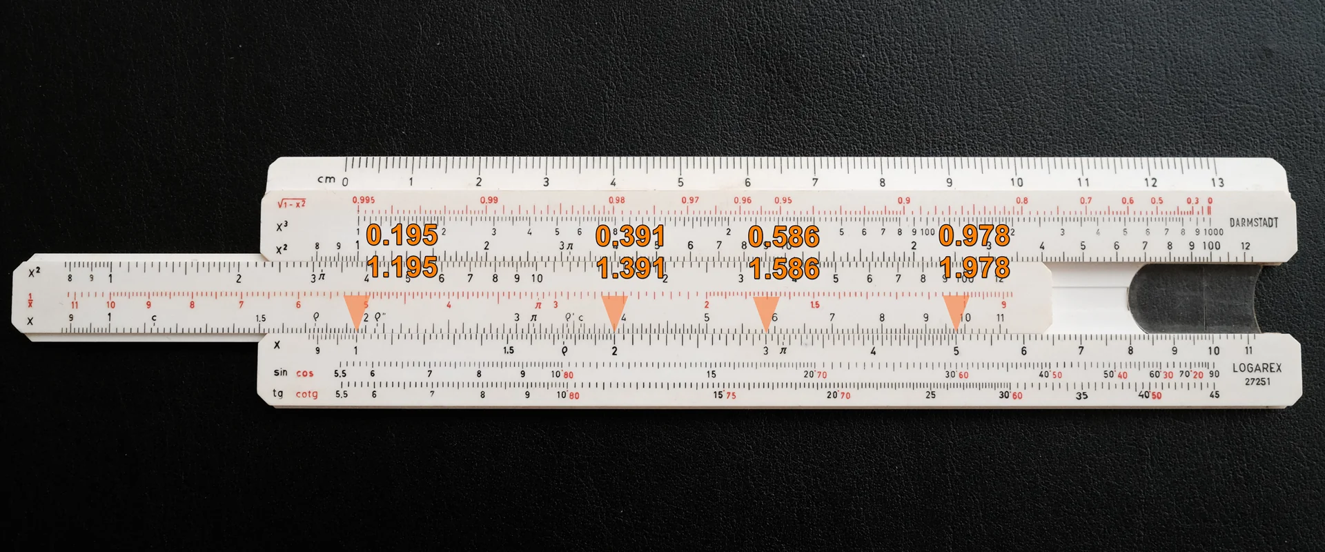 Conversion from electron potential energy (acceleration voltage) to Lorentz factor gamma for 100, 200, 300 and 500 keV. Click on image for higher resolution.
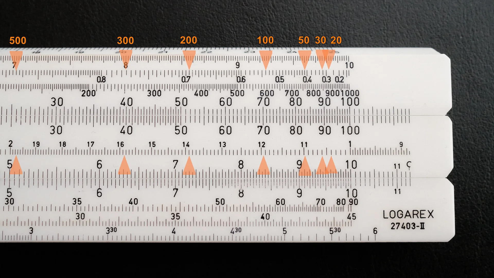 Conversion gamma to speed relative to light. This is the end of 25cm slide rule with quite high magnification which makes reading on this picture easier than by naked eye.
Example: for 100kV we can rad that number above 1 is 0.195 (if we get order of amgnitude right) which is gamma-1 so gamma is 1.195. On second picture we find 1.195 and read 0.55 above.
Summary of slide rule use for real-world problems
We readily reach for smartphones, Excel, or Python for calculations, rendering physical devices almost obsolete. But the humble slide rule, once a ubiquitous tool, still holds its own in specific scenarios. While it won’t compete with calculators in raw speed or precision, its versatile scales offer distinct advantages:
-
Fast Conversions: Unit conversions are fast with the slide rule’s versatile scales. Including ones with inverse proportions. Folded scales could be handy to reduce manipulation and increase overlap of scales when ratio is close to three.
-
Visualizing Relationships: For example exponential growth and decay come alive on the slide rule’s log-log scales, offering a deeper understanding than numerical representations. Combining simple functions, like in the $ \gamma = 1/ \sqrt{1-(v/c)^2} $ is fast.
-
Intuitive Accuracy: Unlike digital abstractions, manipulating the slide rule gives a sense of how fast output changes as input varies and how accurate the result is.
Mastering the slide rule requires initial effort, unlike calculators, and it rewards dedication with unique insights into mathematical relationships. Unlike digital tools that provide single-point results, the slide rule’s visual representation allows you to see how functions interact across a range of values. This dynamic manipulation enables a broader understanding and intuitive grasp of mathematical concepts, making it an excellent educational tool for developing problem-solving skills.