ENG | Atmospheric Calculations for Hobby Weather Stations

Weather stations provide direct measurements like temperature, pressure, and humidity. However, understanding what these values mean in different contexts requires derived calculations. For example, sea level pressure helps meteorologists compare readings across locations at different elevations, while dew point indicates when condensation might occur - important for predicting fog, frost, or precipitation. This article explores the mathematics behind these atmospheric calculations.

However, some conclusions are valid for myself, living in central Europe and considering relatively low altitudes. If you live on a tropical rainforest mountain plateau, some compensations may have different impact :-)

Sea Level Pressure Calculations: Basic Formula

In its simplest form, atmospheric pressure decreases exponentially with altitude. However, real-world conditions are more complex, as air density is influenced by changes in temperature and humidity at different heights. For indoor weather stations, where outdoor conditions might be unknown, the following formula offers a practical approximation:

\[\begin{array}{l c l} P_0 & = & P \cdot \exp\left(\dfrac{g \cdot M \cdot h}{R \cdot T}\right) \\ & = & P \cdot \exp\left(\dfrac{9.80665 \cdot 0.0289644 \cdot h}{8.3144598 \cdot T}\right) \\ & = & P \cdot \exp\left(\dfrac{9.80665 \cdot 0.0289644 \cdot h}{8.3144598 \cdot 288.15}\right) \\ & = & P \cdot \exp\left(\dfrac{h}{29.272 \cdot T} \right) \\ & = & P \cdot \exp\left(\dfrac{h}{8434.7}\right) \end{array}\]

Where

Symbol	Description	Value	Unit
P₀	Sea level pressure		Pa
P	Measured station pressure		Pa
g	Gravitational acceleration	9.80665	m·s⁻²
M	Molar mass of dry air	0.0289644	kg·mol⁻¹
h	Height above sea level		m
R	Gas constant	8.3144598	J·mol⁻¹·K⁻¹
T	Temperature in Kelvins	(288.15)	K

Dry air consists mostly of nitrogen, oxygen, argon and carbon dioxide

Example for P = 100850 Pa

Accuracy analysis: Real vs. “standard” temperature

Temp. [C]	Altitude[m]	Pressure[hPa]	Note
15	250	1038.8	“Standard” outdoor temperature
0	250	1040.5	True outdoor temperature
0	237	1038.8	Altitude giving the same reading

An interesting observation: at altitudes near 300 meters above sea level and an outdoor temperature of 300K (27°C), a 1°C temperature change is equivalent to approximately a 1-meter difference in altitude. In most calculations, actual temperature is often replaced by the standard athmosphere value of 288.15K (15°C). However, local data from my area, Brno, Czechia, suggest an average annual temperature closer to 10°C, making this adjustment less precise for local contexts.

For a reference, pressure changes roughly by one percent per 80 meters of altitude. Pressure in low altitudes is close to 1000.00 Pa. 80m difference cause change of 10hPa. 8m is 1hPa. 80cm is 10Pa (first number after decimal dot).

Be realistic - main source of error will be likely wrong altitude reading of GPS in a tall building, and for a dew point reading of relative humidity or temperature.

Sea Level Pressure Calculations: Temperature Lapse

Everyone’s favorite temperature inversion. Bohemian-Moravian Highlands, September 2020

Now temperature typically changes with altitude, standard rate of change is 6.5K/1km or 0.0065K/m. There might be temperature inversion, we don’t know what weather is below - unless we can observe it from a mountain. There are many ways how approach this - we can adjust temperature by simply taking midpoint between local station and sea level. For 300m altitude, difference between considering this average and local temperature is 0.0065C/m * -150m, which roughly 1C - the same difference as putting station one meter lower.

Nonetheless, there is somewhat overengineered formula which takes variable air density into account, likely for high altitudes or aviation.

\[\begin{array}{l c l} P_0 & = & P \cdot \left(1 - \dfrac{L \cdot h}{T}\right)^{-\dfrac{g \cdot M}{R \cdot L}} \\ & = & P \cdot \left(1 - \dfrac{0.0065 \cdot h}{T}\right)^{-5.25578} \\ & = & P \cdot \left(1 - 2.25577 \cdot 10^{-5} \cdot h\right)^{-5.25578} \end{array}\]

Where:

Symbol	Description	Value	Unit
L	Temperature lapse rate	0.0065	K/m

Accuracy analysis

For comparison, we have some difference between the first equation and two others - this makes about the same error as changing altitude by 70cm for 250m above sea level. If we make error of few percents in this compensation - which already has a small effect - by replacing exponential function by linear, basically nothing happens. On the other hand, both equations have about the same complexity.

Python 3.13.1 (main, Dec  9 2024, 00:00:00) [GCC 14.2.1 20240912 (Red Hat 14.2.1-3)] on linux
Type "help", "copyright", "credits" or "license" for more information.
>>> import math
>>> ### First formula #############
>>> 1008 * math.exp(9.80665 * .0289644 * 250 / (8.3144598 * 288.15) )
1038.3239064868335
>>> ### First formula with temperature lapse compensation for 250m
>>> 1008 * math.exp(9.80665 * .0289644 * 250 / (8.3144598 * (288.15 - 0.0065*250/2) ) )
1038.4109336190797
>>> ### Second formula
>>> 1008 * math.pow(1-0.0065*250/288.15,  -9.80665*.0289644 / 8.3144598 / 0.0065)
1038.41101588332
>>> ### Exponent of second formula
>>> -9.80665*.0289644 / 8.3144598 / 0.0065
-5.2557877405521705

As we can see, beloved temperature inversions that make long periods of heavy overcast in central Europe during winter have very little effect.

Saturation vapor pressure

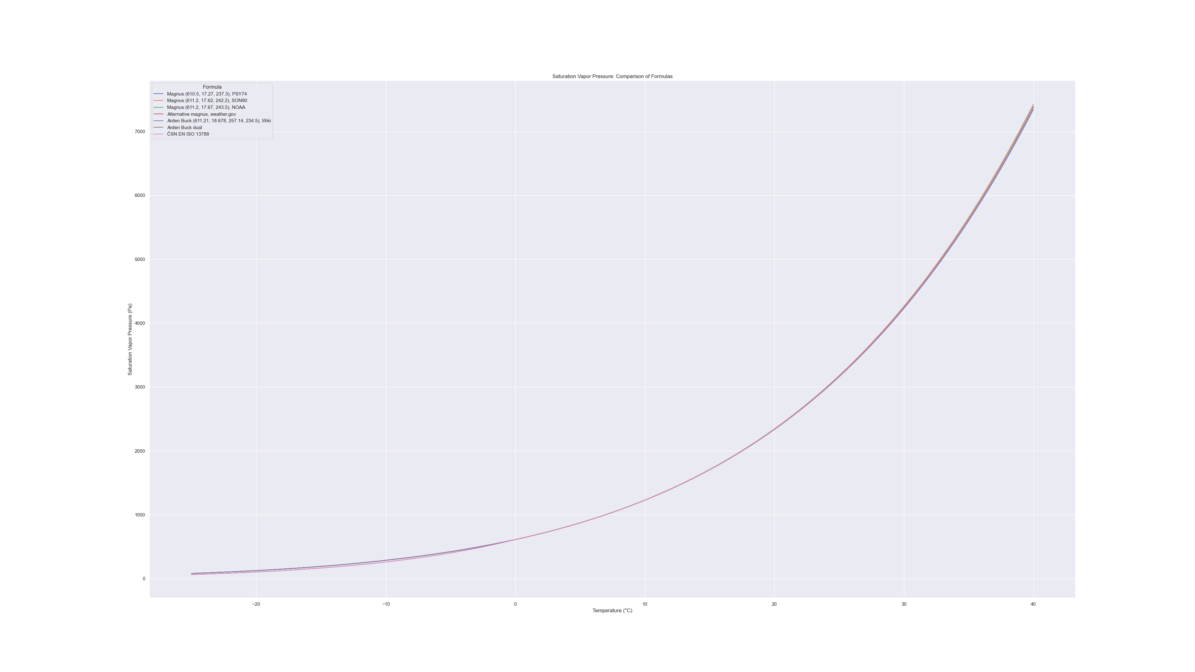
Two common formulas for calculating saturation vapor pressure are the Magnus-Tetens formula and the Arden Buck equation.

While Arden Buck offers greater accuracy, it is more challenging to invert for dew point calculations. The script below compares these formulas and their empirical constants. Notably, some versions account for differences in condensation over water versus ice, resulting in slightly lower saturation vapor pressures at freezing temperatures. It takes more energy for ice to turn into vapor than for water, so saturated pressure over ice is a bit lower.

But state into which water condenses is a bit of mystery as it can remain in state of supercooled water droplets, that freeze on contact with object forming rime ice. Good example of such conditions is a picture on top of this article.

Note that one magnus formula uses different base of ten rather than Euler’s number so one coefficient significantly differs - it can be easily overlooked.

It’s better to run script locally, as differences in the image are negligible.

import numpy as np
import pandas as pd
import seaborn as sns
import matplotlib.pyplot as plt

# Define the functions with varying a, b, c, (d) constants
def magnus_formula(T:float, a:float, b:float, c:float)->float:
    return a * np.exp((b * T) / (c + T))

def saturation_vapor_pressure(T_celsius):
    """Calculate saturation vapor pressure in Pa"""
    return 611 * 10**((7.5 * T_celsius) / (237.3 + T_celsius))

def iso13788(T:float)->float:
    if T<=0.85014:
        return magnus_formula(T, 610.5, 21.875, 265.5) # Mentioned in Arden-buck for freezing temp with large error
    if T<0.84089:
        return 47.18862*T + 609.18998
    return magnus_formula(T, 610.5, 17.269, 237.3)

def arden_buck(T,a=611.21,b=18.678,c=257.14,d=234.5):
    return a * np.exp ((b-(T/d))*(T/(c+T)))

def arden_buck2(T):
    if (T<0):
        return arden_buck(T, 611.15, 23.036, 279.82, 333.7)
    else:
        return arden_buck(T, 611.21, 18.564, 255.57, 254.4)

# Create a map of label to functions with specific a, b, c values
datasets = {
    "Magnus (610.5, 17.27, 237.3), PSY74": lambda T: magnus_formula(T, 610.5, 17.27, 237.7),
    "Magnus (611.2, 17.62, 242.2), SON90": lambda T: magnus_formula(T, 611.2, 17.62, 242.2),
    "Magnus (611.2, 17.67, 243.5), NOAA":  lambda T: magnus_formula(T, 611.2, 17.67, 243.5),
    "Alternative magnus, weather.gov": saturation_vapor_pressure,
    "Arden Buck (611.21, 18.678, 257.14, 234.5), Wiki": lambda T: arden_buck(T),
    "Arden Buck dual": arden_buck2,
    "ČSN EN ISO 13788": iso13788,
}

# Define the temperature range (outdoor conditions)
temperatures = np.linspace(-25, 40, (40+25)*2+1)

# Calculate results and store in a DataFrame
data = {"Temperature (°C)": temperatures}
for label, func in datasets.items():
    data[label] = [func(T) for T in temperatures]

df = pd.DataFrame(data)

# Export DataFrame for further use (optional)
df.to_csv("saturation_vapor_pressure.csv", index=False)

# Melt the DataFrame for Seaborn-friendly format
df_melted = df.melt(id_vars=["Temperature (°C)"], var_name="Formula", value_name="Saturation Vapor Pressure (Pa)")

# Plot using seaborn
sns.set_theme(style="darkgrid")
fig = plt.figure(figsize=(38.4, 21.6))
sns.lineplot(data=df_melted, x="Temperature (°C)", y="Saturation Vapor Pressure (Pa)", hue="Formula")
plt.title("Saturation Vapor Pressure: Comparison of Formulas")
fig.savefig("saturated_vapor_pressure.png")
plt.show()

###########################

with open("saturation_table.py", "w") as f:
    temperatures = np.linspace(-40, 100, (100+40)*2+1)
    f.write("# This file is automatically generated\n\n")
    f.write("# Table of temperature (°C) and saturation pressure (Pa) pairs\n")
    f.write("saturation_table = [\n")
    for t in temperatures:
        f.write(f"    ({t:5.1f}, {arden_buck2(t):7.1f}),\n")
    f.write("]\n")

Here is the high resolution graph:

Sea Level Pressure Calculations: Humidity Compensation

Air density can be affected not only by temperature, but also by ratio of air and water vapor.

To get “virtual temperature” of air which has the same density as humid air, we need to

• Measure temperature, pressure, and relative humidity.
• Calculate saturation vapor pressure, $ e_s $ from temperature.
• Determine actual vapor pressure, $ e = RH / 100 \cdot e_s $ .
• Get virtual temperature, $ T_v = T / (1-e/p \cdot (1-0.622)) $,
• Use virtual temperature instead of measured temperature

The term $ \epsilon=0.622 $ represents the ratio of molar masses of water vapor (18.0153g/mol) to dry air (28.9647g/mol).

Dew or freezing point

The dew-point is the temperature to which the air must be cooled for vapor to reach saturation. As air cannot hold more moisture, it condenses into dew, fog or frost.

To get dew point, we need to get actual vapor pressuren $ e $ by multiplying saturated vapor pressure $ e_s $ by relative humidity. Then we need to find temperature at with this vapor content matches saturation level. In the code below, it’s solved as numeric optimization problem (basically qualified guessing), because I was lazy. In other code it’s inverse look up in the precomputed table.

Specific and absolute humidity

Absolute humidity is a similar concept, but uses volume of air. It’s a bit problematic as air expands with raising temperature.

Specific humidity is the mass of water vapor present in a given mass of air (dry air and vapor mixture), typically expressed in grams of water vapor per kilogram of air. To calculate specific humidity, we use the concept of the mixing ratio, which is the ratio of the mass of water vapor to the mass of dry air in a given volume of air.

Breakdown:

1. Calculate Mixing Ratio: The mixing ratio is the ratio of the mass of water vapor to the mass of dry air. It can be calculated using the formula: \(r = \epsilon \cdot \dfrac{e}{p-e}\) where $ \epsilon $ is the ratio of the molar mass of water vapor to the molar mass of dry air (approximately 0.622), $ e $ is the vapor pressure, and $ p $ is the total atmospheric pressure. This effectively converts molecular ratio into weight ratio.

2. Convert Mixing Ratio to Absolute Humidity: Absolute humidity is then calculated by converting the mixing ratio to grams of water vapor per gram of air (mixture): \(q = \dfrac{r}{1+r}\) Note that in code this is multiplied by 1000 for grams of water per kilogram of air.

All-in-one script

import math
from scipy.optimize import minimize

# https://www.weather.gov/media/epz/wxcalc/vaporPressure.pdf
def saturation_vapor_pressure(T_celsius):
    """Calculate saturation vapor pressure in Pa"""
    return 611 * 10**((7.5 * T_celsius) / (237.3 + T_celsius))

def mixing_ratio(pressure_pa, vapor_pressure_pa):
    """Calculate mixing ratio (dimensionless)"""
    epsilon = 0.62197
    return epsilon * vapor_pressure_pa / (pressure_pa - vapor_pressure_pa)

def virtual_temperature(T_kelvin, pressure_pa, RH):
    """Calculate virtual temperature in K"""
    T_celsius = T_kelvin - 273.15
    e_s = saturation_vapor_pressure(T_celsius)
    e = RH * e_s
    #r = mixing_ratio(pressure_pa, e)
    #return T_kelvin * (1 + 0.61 * r)
    epsilon = 0.62197
    return T_kelvin / (1 - e/pressure_pa*(1-epsilon))

def mean_temperature(T_station, altitude, lapse_rate):
    """Calculate mean temperature of air column below station"""
    return T_station + lapse_rate * altitude * 0.5

def sea_level_pressure(pressure_pa, altitude, T_kelvin):
    """Calculate sea level pressure in Pa"""
    g = 9.80665  # m/s²
    R_d = 287.05  # J/(kg·K)
    return pressure_pa * math.exp((g * altitude) / (R_d * T_kelvin))

def specific_humidity_from_pressures(pressure_pa, vapor_pressure_pa):
    """Calculate specific humidity in g/kg"""
    r = mixing_ratio(pressure_pa, vapor_pressure_pa)
    return 1000 * r/(1.0 + r)

def specific_humidity(T_kelvin, pressure_pa, RH):
    T_celsius = T_kelvin - 273.15
    e_s = saturation_vapor_pressure(T_celsius)
    e = RH * e_s
    return specific_humidity_from_pressures(pressure_pa, e)

def dew_point(T_celsius, RH):
    """Find dew point by reverting saturation_vapor_pressure using numerical optimization."""
    e_s = saturation_vapor_pressure(T_celsius)
    e = RH * e_s  
    result = minimize(lambda T: abs(saturation_vapor_pressure(T)-e), T_celsius, method="Nelder-Mead" )
    if (result.success):
        return result.x[0]
    else:
        return None

# Configuration
altitude = 250.0  # m
pressure = 98500.0  # Pa
#T_measured = 271.15  # K (-2°C)
T_measured = +30 + 273.15
RH = 0.500  # relative humidity
lapse_rate = 0.0065  # K/m

# Temperatures 
T0_standard     = 288.15  # K (15°C)
T_mean_standard = mean_temperature(T0_standard, -altitude, lapse_rate) # compensate for station at 0 -> minus sign
T_mean_measured = mean_temperature(T_measured,   altitude, lapse_rate)
T_virtual       = virtual_temperature(T_mean_measured, pressure, RH)

results = [
    ("Standard temperature", T0_standard),
    ("+lapse              ", T_mean_standard),
    ("Measured temperature", T_measured),
    ("+lapse              ", T_mean_measured),
    ("+lapse & humidity   ", T_virtual)
]

print("\n\033[1mMeasured values\033[0m\n")
print(f"Altitude    : {altitude} m")
print(f"Temperature : {T_measured-273.15:.2f} C")
print(f"Humidity    : {RH*100.0} %")
print(f"Pressure    : {pressure/100:.2f} hPa")

print("\n\033[1mDerived values\033[0m\n")
print(f"Specific humidity : {specific_humidity(T_measured, pressure, RH):.1f} g/kg")
print(f"Dew point         : {dew_point(T_measured - 273.15, RH):.1f} C")

print("\n\033[1mSea level pressure\033[0m\n")
print("| Compensation method  | Temp.    | Pressure    |")
print("|----------------------|---------:|------------:|")

for entry in results:
    print(f"| {entry[0]} | {entry[1]:5.2f} K | {sea_level_pressure(pressure, altitude, entry[1])*0.01:.2f} hPa |")
print("")

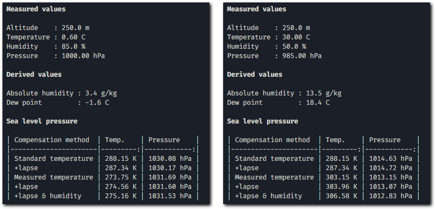Outputs of script with some values for winter and summer.

Conclusion

What significantly affects sea-level pressure calculations is the precise measurement of altitude and the outdoor temperature, especially if it deviates from the standard atmosphere model. There will be noticeable differences between cold winter conditions and summer heat waves.

Compensation for temperature changes with altitude has a minimal effect, as does the impact of relative humidity. Typically, there is rarely more than 1% water vapor in the air, except during hot summer days with occasional thunderstorms.

When I compared data with professional weather stations, they are definitelly compensated for temperature and stations above 550m do not provide information about sea level pressure.

Links

• Wiki -=- Water vapor pressure Equations for saturated vapor pressure, comparison
• Wiki -=- Dew point
• Arden L Buck -=- New methods for Computing vapor pressure … - this compares accuracy of various approximations
• Ametsoc.org -=- glossary
• Weather.gov -=- glossary
• Kurzy.cz -=- Pocitova teplota - (Czech) wind chill temperature, not used here