ENG | Reinventing Logarithms and Slide Rule

Story

I recently found myself using a logarithm by accident when multiplication by $ x^{1/N} $ would have been just as appropriate. It suprised me. I recalled that my mother once taught me about their relation before I learned them at school, when I asked her about mysterious white rule in the drawer.

During a recent visit to my parents, I found this slide rule and realized that it has chipped large part of scales and it’s useful only in limited range. I quickly realized how to perform multiplications with it, but did not realized immediately why it works.

This led me to buying a slide rule and do some research about logarithms, slide rules and history.

Mathematical background for this article

As someone with a background in technical studies from a university, it’s important to note that I do not have a formal education in mathematics. While I possess a solid foundation in technical subjects, my expertise does not extend to the realm of advanced mathematical notation, formal proofs, and the more intricate aspects of mathematical theory. This blog is written from the perspective of a technologist and enthusiast, aiming to demystify mathematical concepts in a way that is accessible and practical, especially for those who, like me, are not mathematicians by training.

Article is based on long conversation with ChatGPT and just a few videos about history. But I believe, it’s somewhat genuine and unique. It describes my understanding of logarithms which got by asking questions how people invented them and even reading parts of Napiers work. Of coarse youtube started recommending relevant videos after I had this article written :) But knowing they exist I would not waste time with this.

Because I don’t want to make this article longer than necessary, there will be some extras. For example programs implementing square root or logarithm or something about my small growing collection of slide rules.

Let’s assume that we know:

• Addition and subtraction
• Multiplications and division
• Powers like x^2, x^3 and calculating square root as inverse operation

And we do not know:

• How to swiftly compute x^N, especially when N is a fraction or a rational number
• How to compute inverse of function above

What troubles us is that manual calculations of large numbers, be it multiplication, division, or even square roots, are excruciatingly slow. Not to mention square root which needs iteratively guessing result, doing squares and readjusting quess based on error.

Cheating

Although computers were nonexistent in the 17th century, I will use programs and tools to drastically shorten the computation time for tables from weeks to milliseconds. This is simply to avoid the tedious work and admit that I struggle to multiply two five-digit numbers without making an error.

Let’s reinvent logarithms

Addition

To perform addition, we can conceptualize numbers as an arithmetic progression from left to right. For example, to add 2 and 3, we combine these distances using calipers or by combining two rulers.

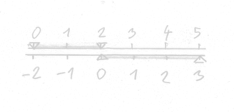
Note that when we use two rulers, every number on top is bigger by two.

Replacing multiplication with addition

To transform multiplication into addition, consider the following example:

\[2^2 \cdot 2^3 = (2 \cdot 2) \cdot (2 \cdot 2 \cdot 2) = 2 \cdot 2 \cdot 2 \cdot 2 \cdot 2 = 2^5 = 2^{2+3} \\ 4 \cdot 8 = 32\]

This can be visualized as a geometric progression where each number is twice as large as its predecessor.

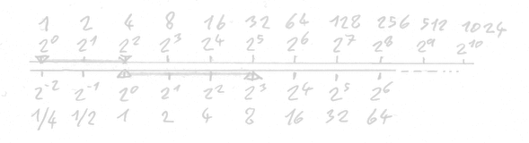
Note that when we use two rulers, every number on top is four times larger.

We have just created our first, rudimentary version of a slide rule 😎

That’s something! However, this method has its limitations, as it only deals with multiples of two. But how to refine our scale, to include more practical numbers such as 3, 5, or 10 ?

We have two options.

• We need to refine the scale using numbers closer to one.
• We may try to find where number 10 lies on this scale more exactly.

Now, it’s insightful to recognize that the square root of two, denoted as 2^(1/2), fits perfectly between 1 and 2 in our geometric progression. This is because 2^(1/2), when squared (multiplied by itself), equals two. To refine our scale even further, we can calculate 2^(1/4), representing the square root of 2^(1/2).

In the context of geometric progression, the number that lies exactly halfway between 8 and 16 (or any two numbers) is called the geometric mean. The geometric mean, generally defined as $ \sqrt{a \cdot b} $ , in this case, is:

\[\sqrt{8 \cdot 16} = \sqrt{2^3 \cdot 2^4} = \sqrt{2^{3+4}} = \sqrt{2^7} = 2^{7/2} = 2^{3.5} = 2^3 \cdot \sqrt{2}\]

This calculation shows how 2^(7/2) seamlessly integrates into our scale, maintaining the uniformity of the geometric progression.

Historical note: Interestingly, the method for finding square roots has been known since Babylonian times. However, the rationale behind why this formula works wasn’t established until Newton’s development of differential calculus. Check this link https://thepalindrome.org/p/how-did-the-babylonians-know-2-up or search The Babylonian square-root algorithm, Hero(n)’s method, or Newton–Raphson method

Refining scale by smaller number(s)

We have several options, two of them seem somewhat reasonable:

• Stick with square roots. Actually, this is a pretty bad idea. Unless you are a masochist or you can use a computer. Calculating square root is iterative process, where each iteration includes two divisions and roughly doubles the precision from initial guess. Multiplying numbers with many decimal places is not convenient neither. Manual calculation would take hours.

• Opt for a number close to one that simplifies multiplication, like 1.1, 1.01, 1.001. Multiplying by 1.1, for example, means multiplying a number by 0.1 and then adding it to the original number. This process involves shifting the number by one digit and then rounding the last digit. We can choose 0.9 or 0.99 as well and use similar trick. This really saves time.

Step  Number (1.1)  Number (0.9)
0     1.00000       1.00000
       .10000      - .10000
      ───────       ─────── 
1     1.10000       0.90000
        11000      -   9000
      ───────       ───────
2     1.21000       0.81000
        12100      -   8100
      ───────       ───────
3     1.33100       0.72900
        13310      -   7290 
      ───────       ───────
4     1.46410       0.65610
        14641             ┊
      ───────
5     1.61051
┊           ┊
6     1.77156
7     1.94872
8     2.14359
9     2.35795
10    2.59374
11    2.85312
12    3.13843
13    3.45227
14    3.79750
15    4.17725
16    4.59497
17    5.05447
18    5.55992
19    6.11591
20    6.72750
21    7.40025
22    8.14027
23    8.95430
24    9.84973
25    10.8347

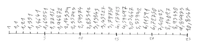
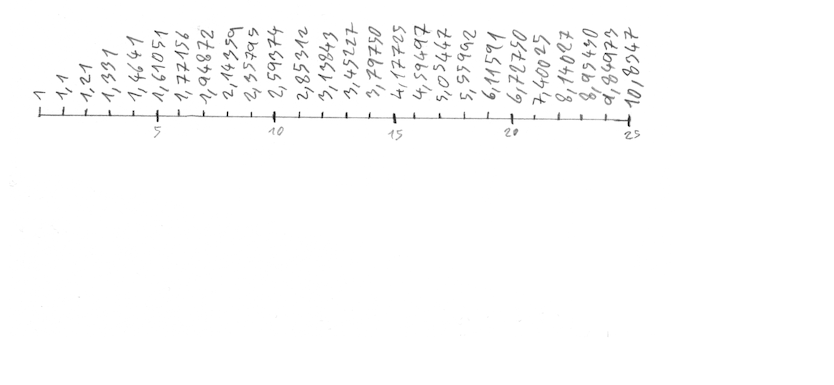
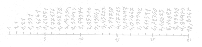Image shows geometric progression of 1.1 which has finer resolution than geometric progression of 2

Finding position of ten (as an example)

Good. We made some progress. But now, how do we find the position of 10 and maybe do it more exactly?

For instance, we may want to stretch our slide rule scales based on the Nth power of two and Nth power of 1.1 to match. And we want to place ten maybe 10cm or 25cm far from one.

Well. For geometric progression of 1.1, it’s between 24 and 25. Obviously closer to 24.

There are two obvious solutions:

1. Interpolation

 x      y
24   9.84973
25  10.8347

dx = 1 
dy ≈ 10.83 - 9.85 ≈ 0.98 ≈ 1

x  = x1 + dx * (y-y1)/dy
   = 24+(10-9.85) 
   = 24.15

2. Interval subdivision

24 1/2                      sqrt(9.84973*10.8347) = 
                            sqrt(9.84973*9.84973*1.1) = 
                            9.84973*sqrt(1.1)     = 10.3305
24 1/4                      sqrt(9.84973*10.3305) = 10.0873
24 1/8                      sqrt(9.84973*10.0873) = 9.96781
24 (1/4+1 /8)/2 = 24 3/16   sqrt(9.96781*10.0873) = 10.0274
24 (1/8+3/16)/2 = 24 5/32   sqrt(9.96781*10.0274) = 9.99756

24 5/32 = 24.15625

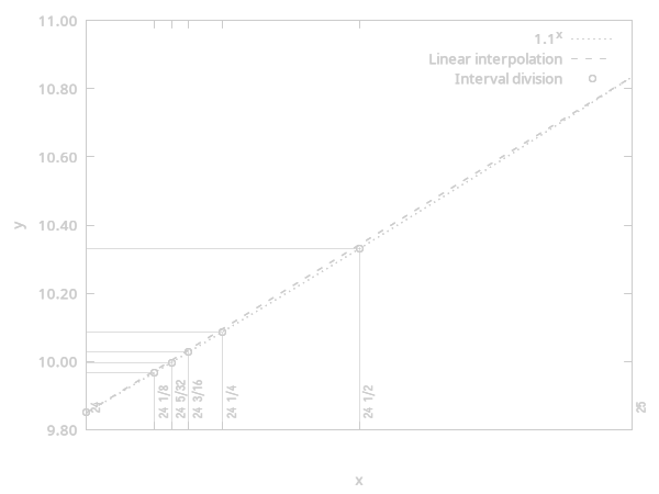
It’s a pretty good match, with an error of only 0.025%. Today, we have a convenience of verifying result using a calculator: 1.1^(24+5/32) = 9.99751

The same example for powers of two

Because we don’t have enough data points for powers of two, linear interpolation would not work so well - it gives us result

dx =  (4-3) = 1
dy = (16-8) = 8

x  = x1 + dx * (y-y1)/dy =
   = 3 + 1 * (10-8)/8 =
   = 3 + 1/4 =
   = 3.25

Ok, let’s do interval subdivision for that.

3                               8
4                               16
3 1/2                           sqrt(8*16) = 8*sqrt(2) = 11.3137
3 1/4                           sqrt(8*11.3137)        = 9.51365
3 (1/2+1/4)/2 = 3 (3/8)         sqrt(11.3137*9.51365)  = 10.374
3 (1/4+3/8)/2 = 3 5/16          sqrt(10.374*9.51365)   = 9.93452
3 (5/16+3/8)/2 = 3 11/32        sqrt(9.93452*10.374)   = 10.1519
3 (11/32+5/16)/2 = 3 21/64      sqrt(9.93452*10.1519)  = 10.0426
3 (21/64+5/16)/2 = 3 41/128     sqrt(10.0426*9.93452)  = 9.98841
3 (41/128+21/64)/2 = 3 83/256   sqrt(10.0426*9.98841)  = 10.0155
3 (83/256+41/128)/2 = 3 165/512 sqrt(10.0155*9.98841)  = 10.0019

3 165/512 = 3.32227

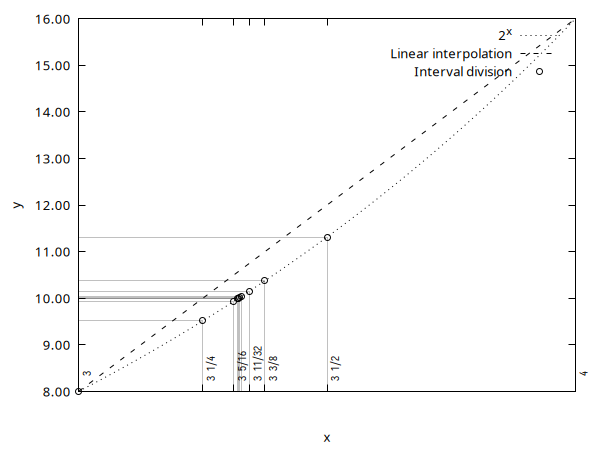
Now we have error 0.019% or two microns at 10cm scale, but using linear interpolation is not accurate and we started with longer interval.

Third solution will be shown later, once we build foundains.

Understanding Scale Variability

Itriguingly, we managed to calculate that if we use base 2 for powers, 10 is 3.322 units far, and we if use base 1.1 it’s 24.15 units far. If we use base 10 it’s one unit far. It’s worth noting, that if we change powers of two to powers of four, a distance to reach any number halves and when we use square root of two it doubles. We may use this to stretch or compress our scales as we want to match each other, because size of “unit” is arbitrary.

This becomes evident when we look at the picture showing how the number 10 is represented in different bases:

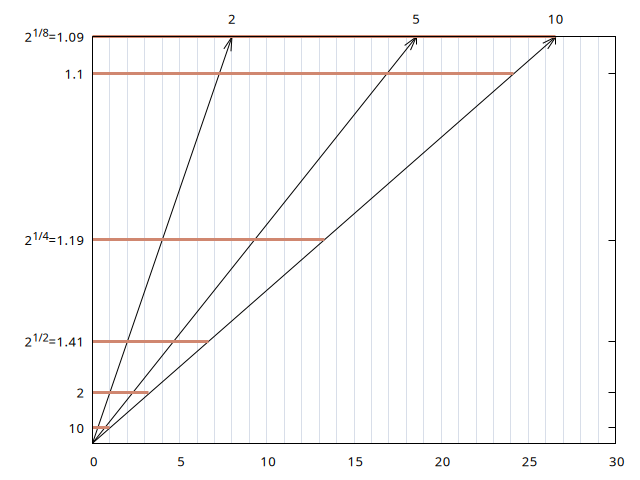
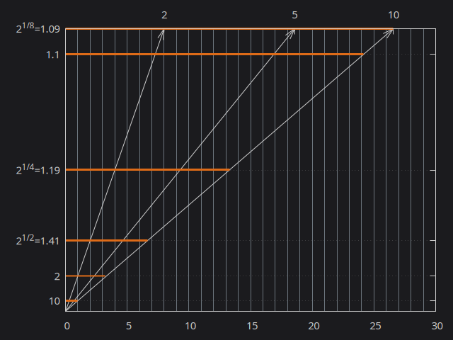
• Base 10: As expected, the number 10 is just 1 unit away.
• Base 2: The number 10 is represented as 3.322 units.
• Base 1.1: In this base, the distance stretches to 24.15 units.
• Base 2^(1/8): The Number 10 is represented as 26.58 units (8x3.322)

Constructing a Practical Slide Rule

We can strategically combine approaches to create a more useful slide rule:

• Starting with a Smaller Base: Opting for a base number like 1.01 (instead of 1.1) allows for more precise refinement of the scale. Although this initially means more simple calculations (additions and shifts), the payoff is greater accuracy in the long run, particularly for interpolations.

• Utilizing square roots for larger gaps: When our scale spans a wide range, employing square roots can be effective. For instance, the square root of 1.1 (approximately 1.04881) can be multiplied by 1.01 to infill our scale with additional values, enriching our table of powers for 1.1 by twice more values.

• Simplifying Calculations with Fractional Exponents: A practical way to fractional exponents is to break them down into their integer and fractional parts. For example, 2^3.32227=10 can be divided into 2^3=8 times 2^0.32227=1.25. This approach reveals a consistent pattern where each successive number is 1.25 times larger than the one before it (e.g., the progression from 1 to 1.25, 2 to 2.5, 4 to 5, 8 to 10, etc.).

Now let’s make slide rule version two assuming that we know position of 10, and prime numbers 2,3,7. We know that we can take a compass, take distance between 1-2 and start adding numbers such as 2*2=4, 4*2=8, 8*2=16, 10*2=20, 10/2=5, 5/2=2.5, 2.5/2=1.25, 3*2=6, 6*2=12, 3/2=1.5, 7*2=14, 7/2=3.5, 3.5/2=1.75, 3*3=9, 6*3=18, 3*5=15, 15/2=7.5, 9/2=4.5, 4.5/2=2.25, 2.25/2=1.125, 6/5=1.2 7/5=1.4, 9/5=1.8, 12/5=2.4, 14/5=2.8, 16/5=3.2,… . Then we can divide all numbers between 10 and 20 by 10 by basically substracting 10 and add new prime numbers 11, 13, 17, 19, … or we can simply start using interpolation.

Note that we already used relations between multiplication and addition to find positions of many numbers geometrically.

Side Note: Real World Slide Rules

Let’s look at the Logarex 27103, a basic but functional slide rule, to see how these principles are applied in real-world tools.

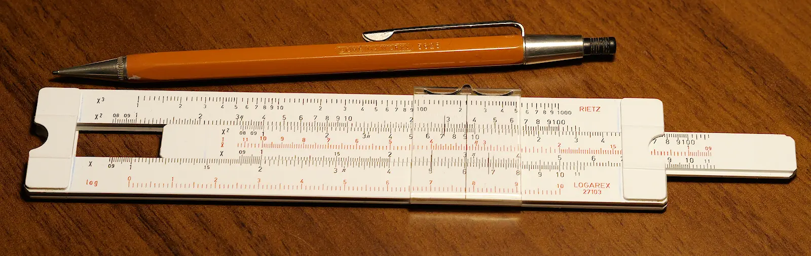Logarex 27103 Rietz 10cm slide rule from May 1967

This slide rule already has multiple functions: there are two pairs of scales x (more accurate) and x^2 (more comfortable) used for multiplication. They can be used for powers of two and square root because as we mentioned, these scales are twice longer. For the same reason there’s a scale x^3. Then there is inverted/reciprocal scale 1/x and linear scale log(x). Hidden fuction is in hairlines used for kW <-> HP conversion (1.36x, Europe used different horse power than US) and conversion between circle diameter and circle area (S=πr² -> S=π/4·d²) so it matches distance between π and 4 on x^2 scale. Scales are extended a bit so it works on both ends. This design is very common on European slide rules.

Slider rules differ in

• materials (pearwood, bamboo, celluloid, epoxy resin, plastics, aluminum)
• manufacturing quality
• number and arangement of scales (Aristo Hyperlog 0972 has 31 of them, Pickett N4 has 34 scales)
• length (10cm/4inch, 12.5cm/5”, 15cm/6”, 25cm/10”, 50cm/20” )
• aesthetics, clarity and legibility

I would say most European ones are either System Rietz or System Darmstadt which dictates their scale arrangement. It seems that duplex slide rules with more scales are not common until sixties.

There are some special slide rules with specific applications such as geodetics and navigation, machine shops, design of reinforced concrete constructions, …

Maybe there will be article about them.

What is logarithm?

Think of a logarithm as the opposite of exponentiation. It tells us how many times we need to multiply a base number by itself to get desired result. For instance, in the equation

\[\begin{align*} 2^3=8 \\ log_{2}8 = 3 \end{align*}\]

the logarithm to the base 2 of 8 is 3, because we multiply 2 by itself three times to get 8.

Decadic logarithm to the base 10 is typically written as $ \log $, whereas natural logarithm has base $ e = 2.7182818284590… $ and is written as $ \ln $.

So far, I avoided term logarithm and used distance in geometric progression instead.

Logarithmic identities

Inverse Function

Identity:

\[b^{log_bx} = x\]

Example:

\[2^{log_28} = 2^3 = 8\]

The Power Rule

Identity:

\[log_b{x^y} = y \cdot log_b{x}\]

Examples:

\[\begin{gather*} \log_2(8) = \log_2(2^3) = 3 \cdot \log_22 = 3 \cdot 1 = 3 \\ \log_2(1/8) = \log_2(2^{-3}) = -3 \\ \log_2(8^2) = 2 \cdot \log_2(8) = 2 \cdot 3 = 6 \\ \log_2(10^3) = 3 \cdot \log_2(10)=3 \cdot 3.322 = 9.966 \end{gather*}\]

The last example is not that obvious, but $ 2 \cdot 2 \cdot 2 \cdot 2 \cdot 2 \cdot 2 \cdot 2 \cdot 2 \cdot 2 \cdot 2 = 1024 $ and it term of geometric progression, 1000 is three times further than 10.

The Product rule

Identity::

\[\log_bxy = \log_bx + \log_by\]

Because:

\[b^{\log_bx+\log_by}= b^{log_bx} \cdot b^{\log_by} = x \cdot y\]

Example:

\[\begin{gather*} 2^{2+3} = 2^2 \cdot 2^3 = 2^{\log_24+\log_28}= 2^{\log_24} \cdot 2^{\log_28} = 4 \cdot 8 \\ \log 0.0123 = \log (1.23 \cdot 10^{-2}) = \log1.23 + \log10^{-2} = \log1.23 - 2 \end{gather*}\]

The Quotient Rule

Identity:

\[\log_b \frac{x}{y} = \log_bx - \log_by\]

Example:

Consider simplifying fraction

\[\frac{2^5}{2^2} = \frac{2 \cdot 2 \cdot 2 \cdot \cancel{2 \cdot 2}}{\cancel{2 \cdot 2}} = 2^3 = 2^{5-2}\]

Applying the Quotient Rule, we calculate the logarithm:

\[\log_2(\frac{2^5}{2^2}) = \log_2(2^5) - \log_2(2^2) = 5 - 2 = 3\]

Changing base of logarithm

Identity:

\[\log_{newBase}(x) = \frac {\log_{oldBase}(x)} {\log_{oldBase}(newBase)}\]

Example:

\[\log_{10}8 = \frac{\log_2(8)}{\log_{2}(10)} = \frac{3}{3.322} = 0.903\]

Do you recall this picture?

Changing base of logarithm is basically the same as multiplying by a scalar. To change the base of logarithm, we can basically stretch scales to match each other. If we know that log(2,8)=3, log(2,10)=3.322 and log(10,10)=1, we can find that log(10,8) = log(2,8) * log(10,10) / log(2,10) = 3 * 1 / 3.322 = 0.903

julia> 3 / 3.322
0.9030704394942806

julia> log(10,8)
0.9030899869919434

How to calculate logarithm on a simple computer

Here’s the promised third solution.

Remember our tables of geometric progression for 1.1, 1.01, 1.001? We can precompute logarithms of these numbers and use identities we introduced.

For example we can write 50 as

\[50 = 10^a \cdot 1.1^b \cdot 1.01^c \cdot 1.001^d \cdot 1.0001^e \cdot ...\]

First, obviously

\[50 = 5.0 \cdot 10^1\]

Then we need a table with exponents and powers of progressivelly smaller numbers such as 1.1, 1.01, 1.001, … and their decimal logarithms which grow in a direct proportion to exponent.

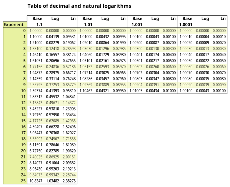
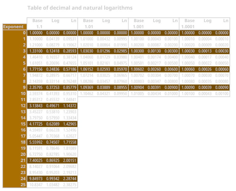
Now we need to decompose 5. From the first table we can find that first number below five is 4.59497 which is 1.1^16. Now we can divide 5 by 4.59497 which equals to 1.08815 and find entry below this number. It’s 1.08286 which is 1.01^8 and something. We will continue by 1.08815/1.08286=1.00489 and so on.

\[\begin{align*} 50 &= 10^1 \cdot 1.1^{16} \cdot 1.01^{8} \cdot 1.001^4 \cdot 1.0001^8 \\ \log(50) &= \log(10^1 \cdot 1.1^{16} \cdot 1.01^{8} \cdot 1.001^4 \cdot 1.0001^8) \\ \log(50) &= \log(10^1) + \log(1.1^{16}) + \log(1.01^8) + \log(1.001^4) + \log(1.0001^8) \\ \log(50) &= 1 + 16 \cdot \log(1.1) + 8 \cdot \log(1.01) + 4 \cdot \log(1.001) + 8 \cdot \log(1.0001) \end{align*}\]

Line above is more sensitive to rounding error, but it makes calculation even more simple. If we know logarithms of 1.1, 1.01, … to more decimal places, we need only few known logarithms and rougly one division per decimal place.

\[\begin{align*} \log(50) &= 1 + 0.66228 + 0.03457 + 0.00174 + 0.00035 \\ \log(50) &= 1.69894 \end{align*}\]

Verification

[pavel -=- ~] julia
               _
   _       _ _(_)_     |  Documentation: https://docs.julialang.org
  (_)     | (_) (_)    |
   _ _   _| |_  __ _   |  Type "?" for help, "]?" for Pkg help.
  | | | | | | |/ _` |  |
  | | |_| | | | (_| |  |  Version 1.9.3 (2023-08-24)
 _/ |\__'_|_|_|\__'_|  |  FreeBSD port lang/julia build
|__/                   |

julia> 10 * 1.1^16 * 1.01^8 * 1.001^4 * 1.0001^8
49.9962787682547

julia> 1 + 0.66228 + 0.03457 + 0.00174 + 0.00035
1.6989400000000001

julia> 10^(1 + 0.66228 + 0.03457 + 0.00174 + 0.00035)
49.996545742482354

julia> 10^(1 + 0.66228 + 0.03457 + 0.00174 + 0.00039)
50.00115080658723

julia> log(10,50)
1.6989700043360185

julia> log(10, 10^1) + log(10, 1.1^16) + log(10, 1.01^8) + log(10, 1.001^4) + log(10, 1.0001^8)
1.6989376809249173

julia> 1*log(10, 10) + 16*log(10, 1.1) + 8*log(10, 1.01) + 4*log(10, 1.001) + 8*log(10, 1.0001)
1.6989376809249175

Natural logarithm is more complicated for numbers above 10, we can’t just use position of decimal point.

TODO: Python or C++ program, links to extras

Summary

In this article, we explored concept of exponentiation, logarithms, motivation behind them and construction of basic slide rule which exploits their property of converting multiplication into addition.

Article does not cover any advanced functions of later slide rules, such as using log-log scales for computing fractional exponents, trigonometric functions or folded scale.

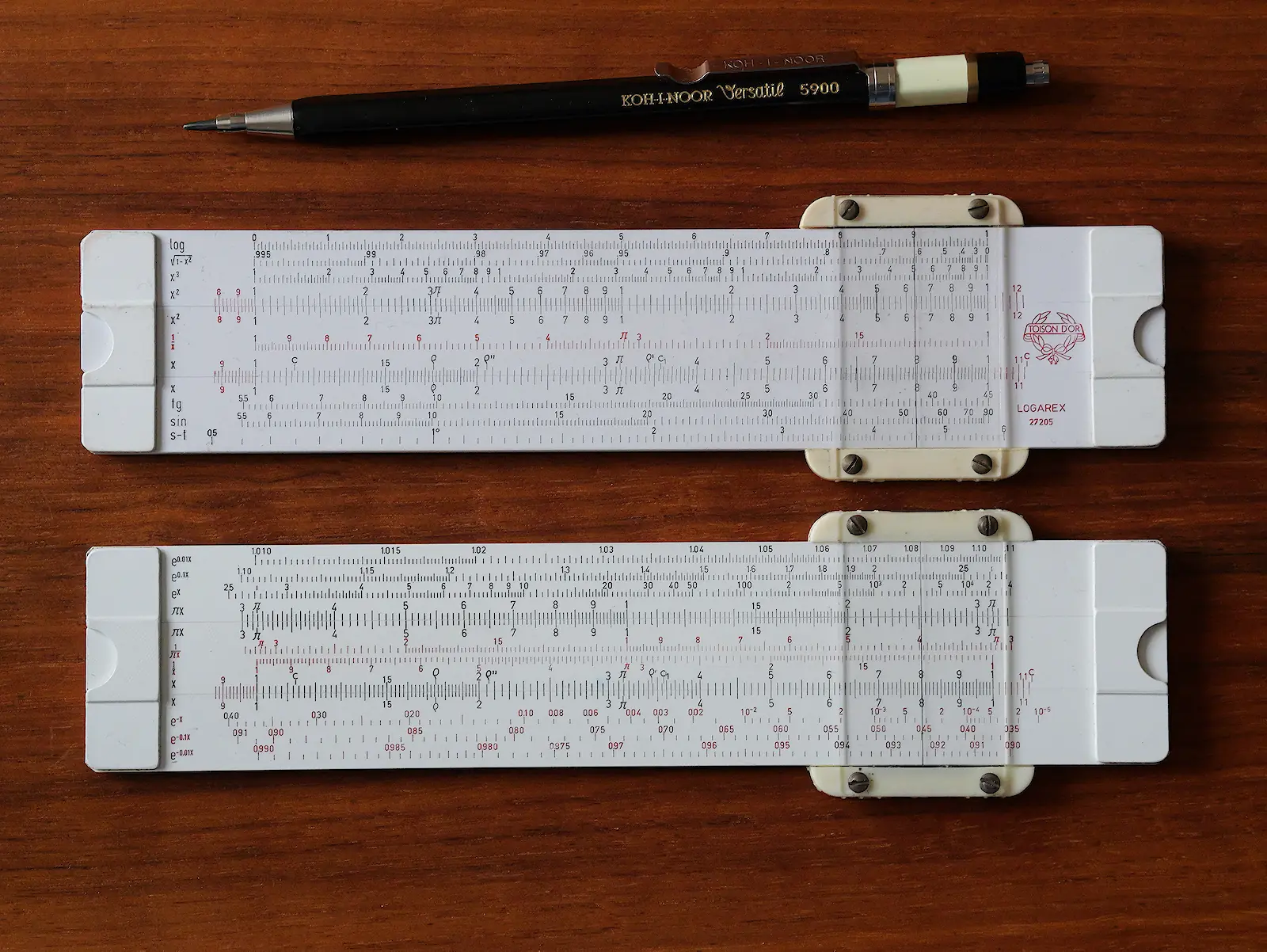Logarex 27205 duplex 12.5cm slide rule from Jan 1962 (other has no date). The most advanced “pocket” slide rule made in Czechoslovakia

This might be covered in future article about slide rules, but I guess I cannot add much to slide rule manuals.

On the other hand it might be nice to to reinvent log-log scales and how to calculate trigonometric functions. Tables were known in 17th century and actually Napier made table of logarithms and sines for all numbers from 0 to 90 degree with resolution of arc minute, thus 5400 entries on 180 pages (30 entries per page).

In my opinion, slide rule has many drawbacks in computer era:

• Inaccuracy (tables can be used if required)
• It’s somewhat slow (relative to calculator)
• It’s necessary to keep track of order of magnitude
• When result of multiplication is close to 10, it’s hard to estimate which direction to use
• There’s a room for errors
• Some “advanced tasks” require practise

But even then there are some advantages

• It can be used as “multiplication table” for unit conversions, direct proportions and inverse proportions. I think this is quite unique and having “folded scales” is vital.
• The same is true for log-log scales (exponential growth and decay)
• User has some sense of accuracy

The following part is unfinished and will likely be part of the separate article

Historical context

Year	Author	Achievement
1614	John Napier	Work about logarithms published, “Mirifici Logarithmorum Canonis Descriptio”
1617	Henry Briggs	Table of decimal logarithms for all integer values from 1 to 1000 with 14 digits precision
1620	Joost Bürgi	Independent publication of logarithms, “Arithmetische und Geometrische Progress Tabulen”
1624	Edmund Gunter	Developed a logarithmic scale, known as Gunter’s rule
1630,32	William Oughtred	Invention of the circular and straight slide rule
1722	Warner	Two and three decade scales
1748	Leonhard Euler	Introduction of the natural logarithm, based on the number ‘e’
1755	Everard	Inverted scale
1775	John Robers	Development of slide rule cursor
1815	Peter Mark Roget	Invention of Log log scale principle, useful for fractional exponents
1859	Amédée Mannheim	Standardization of the modern slide rule (A,[B,C],D scales)
		System Rietz
1933	Hubert Boardman	Differential trigonometrical and log log scales (used in Britain)
1934		System Darmstadt (adds P and LL1,LL2,LL3 scales on back of slider)
1976	Slide rule made obsolete by cheap calculators
1981	Last year Logarex produced slide rules

Sources: wiki, chatgpt, British Thornton AA010 slide rule manual.

Useful links

Link	Description
The Math Doctors - Evaluating Square Roots by Hand	Article describing three methods evaluating square root
Ciaran McEvoy - Logarithms: why do they even exist?	Video about history of logarithms
Tarek Said - The History of the Natural Logarithm - How was it discovered?	Video about history of logarithms with focus on natural logarithms
Wikipedia - History of logarithms	Wikipedia page about history of logarithms
Logaro.cz - Historie Logarexu pohledem pamětníka	Interview with employee of Logarex slide rule factory
Math Vault - Logarithm: The Complete Guide (Theory & Applications)	In-depth article about logarithms and identities
The Oughtred Society	Page Dedicated to the preservation and history of slide rules and other calculating instruments
The Oughtred Society - Slide rule reference manual	PDF Book about slide rules
John Savard’s Home Page	Page dedicated to slide rules, math, computers
Dr. Steve Arar - An Introduction to the CORDIC Algorithm	How computers evaluate trigonometric functions
Logaro.cz - Historie Logarexu pohledem pamětníka	Czech Interview with employee of Logarex slide rule factory
Kreteni - Logaritmické pravítko	Czech slide rule manual converted to HTML
Derek Ross - Slide Rule Calculations by Example	Basic guide to all scales
Following the Rules	Comprehensive page about slide rules and logarithms.